Chapter Nine: Support Vector Machines

Applied Problems

Load in the standard libraries

import pandas as pd
import numpy as np
import random
import os

import matplotlib.pyplot as plt
import seaborn as sns

Set the seed for reproducibility

np.random.seed(101)

Problem Four

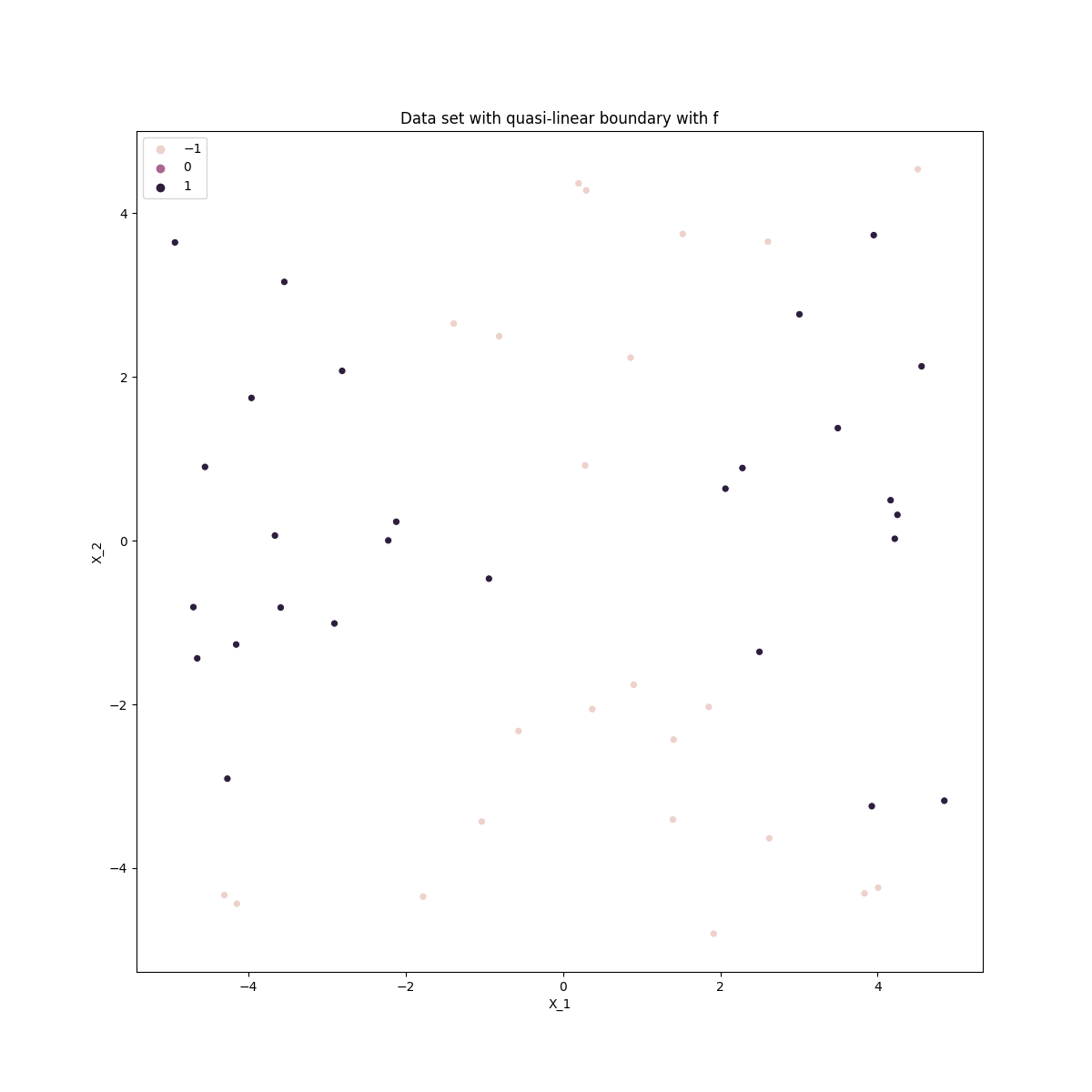
To generate the non-linear data we use the following code,

## Define the two predictors and create a dataframe to pass to models
x_1 = 10*np.random.uniform(size=50) - 5
x_2 = 10*np.random.uniform(size=50) - 5
X = np.column_stack((x_1, x_2))

## Create the labels
y = []
for i in range(len(x_2)):
    ## Non linear function
    arg = x_1[i]**2 - x_2[i]**2
    if arg > 0:
        y.append(1)
    else:
        y.append(-1)
y = np.array(y)

We can now plot this data,

## Plot the data with labels
fig, ax = plt.subplots(1,1,figsize=(12,12))
sns.scatterplot(x=x_1, y=x_2, hue=y, ax=ax)

ax.set_xlabel('X_1')
ax.set_ylabel('X_2')
ax.set_title('Data set non-linear boundary')

plt.show()
plt.close()

PRSS Ridge

Linear kernel

Fitting this plot with a linear kernel we will use cross validation to find the best value of the cost function which minimizes the test error.

from sklearn.svm import SVC
from sklearn.model_selection import cross_validate

## Instantiate the linear SVC
lin_svm = SVC(kernel='linear')

## Set baseline score
best_score = 0

## Set empty list for storing training and test scores
cv_score_C_test = []
cv_score_C_train = []
C_values = np.arange(0.001, 5, 0.001)
# C_values = [np.power(10.0,x) for x in np.arange(0,7,1)]
for c in C_values:
    print(c)
    lin_svm.set_params(C=c)
    scores = cross_validate(lin_svm, X, y, return_train_score=True, n_jobs=-1)
    print(scores['test_score'].mean())
    print(scores['train_score'].mean())
    cv_score_C_test.append(scores['test_score'].mean())
    cv_score_C_train.append(scores['train_score'].mean())

    ## If the iteraction is the current best perfomer, save the parameters and model
    if scores['test_score'].mean() > best_score:
        best_score = scores['test_score'].mean()
        lin_svm.fit(X,y)
        best_model = lin_svm
        best_C_value = c

print('Best value of cost (C): ', round(best_C_value,3))
print('Best test set score: ', round(best_score, 3))

Best value of cost (C):  4.763
Best test set score:  0.68

Plot the results of this

fig, ax1 = plt.subplots(nrows=1, ncols=1, figsize=(12,6))
ax1.plot(C_values, cv_score_C_test, label='test score')
ax1.plot(C_values, cv_score_C_train, label='train score')

ax1.set_xlabel('C')
ax1.set_ylabel('Score')
ax1.set_title('Model performance for gamma')
ax1.legend(fontsize = 'large')
ax1.set_xscale('log')

plt.savefig(os.path.join(IMAGE_DIR, 'q4_linear_C.png'))
plt.show()
plt.close()

PRSS Ridge

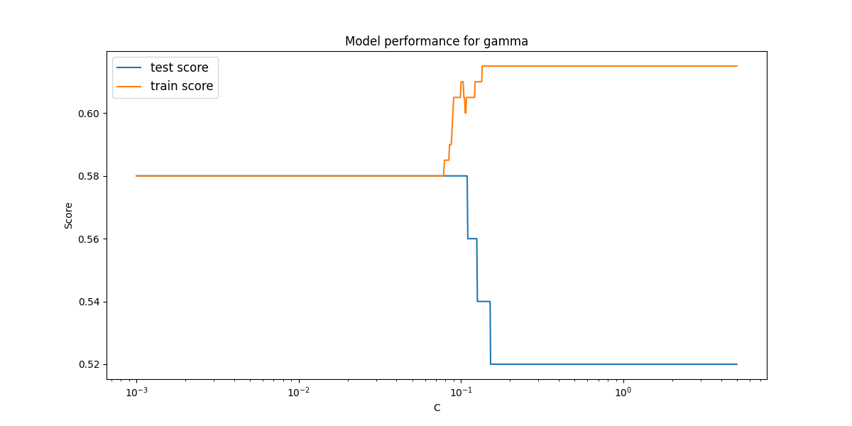
This is a very poor performing model, with an extremely poor test score. Even the training score levels out at a value of $\approx 0.62$. This is to be expected as we are attempting to fit a linear hyperplane to a non-linear decision value.

Polynomial kernel

For the polynomial kernal we cross validate and score in a similar way, however there are more hyperparameters to optimize. THe bet course of action is to use a random grid search the find the most optimal value however we will iterate over the hyperparameters individually to generate some plots. For each polynomial degree up to five we will find the best gamma value then find the best cost value. As the two are not indepenedent this may not represent the most optimal model but should be good for demonstration. We use a very similar model as the linear model above with different hyper parameters.

def plot_score_vs_param(model,X, y, para, param_values):
    ## Set baseline score
    best_score = 0

    ## Set empty list for storing training and test scores
    cv_score_test = []
    cv_score_train = []
    values = param_values
    # C_values = [np.power(10.0,x) for x in np.arange(0,7,1)]
    for val in values:
        print(para + '_value: ' + str(val))
        if para == 'C':
            model.set_params(C=val)
        if para == 'gamma':
            model.set_params(gamma=val)
        if para == 'degree':
            model.set_params(degree=val)
        scores = cross_validate(model, X, y, return_train_score=True, n_jobs=-1)
        print('test score: ', scores['test_score'].mean())
        print('train score: ', scores['train_score'].mean())
        cv_score_test.append(scores['test_score'].mean())
        cv_score_train.append(scores['train_score'].mean())

        ## If the iteraction is the current best perfomer, save the parameters and model
        if scores['test_score'].mean() > best_score:
            best_score = scores['test_score'].mean()
            model.fit(X,y)
            best_model = model
            best_value = val

    print('Best value of cost (C): ', best_value)
    print('Best test set score: ', round(best_score, 3))

    results = {}
    results['best_test_score'] = best_score
    results['best_model'] = best_model
    results['best_value'] = best_value
    results['train_scores'] = cv_score_train
    results['test_scores'] = cv_score_test

    return results

    ## Instantiate the SVC with polynomial kernel
    ## Maximum iteractions set as finding optimal solution will be difficult for wrong fits.
    poly_svm = SVC(kernel='poly', max_iter=10000000)

    ## Set the values to iterate over
    ### Polynomial degrees
    degree_values = [1,2,3,4,5,6]
    ### Gamma Values
    # gamma_values = np.arange(0.001, 1, 0.01)
    gamma_values = [np.power(10.0,x) for x in np.arange(-7,7,1)]
    ### Cost Values
    # C_values = np.arange(0.001, 5, 0.01)
    C_values = [np.power(10.0,x) for x in np.arange(-7,7,1)]

    ## Set up figure to plot train, test scores
    fig, axs = plt.subplots(nrows=len(degree_values), ncols=2, figsize=(12,32))
    ## For each degree produce a new row in the plot
    for idx, deg in enumerate(degree_values):
        print("Degree: ", deg)
        ## Update model with new polynomial degree
        poly_svm.set_params(degree=deg)
        ## Perform CV with gamma values
        gamma_results = plot_score_vs_param(poly_svm, X, y, para='gamma', param_values=gamma_values)
        ## Update model with best gamma value
        poly_svm.set_params(gamma=gamma_results['best_value'])
        ## Perform CV with C values
        C_results = plot_score_vs_param(poly_svm, X, y, para='C', param_values=C_values)

        ## Update axes with new plots
        axs[idx,0].plot(gamma_values, gamma_results['test_scores'], label='test score')
        axs[idx,0].plot(gamma_values, gamma_results['train_scores'], label='train_score')
        axs[idx,0].set_xlabel('gamma')
        axs[idx,0].set_ylabel('Score')
        axs[idx,0].set_title('Model performance for gamma (Degree {})'.format(deg))
        axs[idx,0].legend(fontsize = 'large')
        axs[idx,0].set_xscale('log')

        axs[idx,1].plot(C_values, C_results['test_scores'], label='test score')
        axs[idx,1].plot(C_values, C_results['train_scores'], label='train_score')
        axs[idx,1].set_xlabel('C')
        axs[idx,1].set_ylabel('Score')
        axs[idx,1].set_title('Model performance for C (Degree: {0}, gamma: {1:.2})'.format(deg,gamma_results['best_value']))
        axs[idx,1].legend(fontsize = 'large')
        axs[idx,1].set_xscale('log')

    plt.tight_layout()
    plt.savefig(os.path.join(IMAGE_DIR, 'q4_poly_cv_plots.png'), dpi = 300)
    plt.show()
    plt.close()

This gives the following plot,

PRSS Ridge

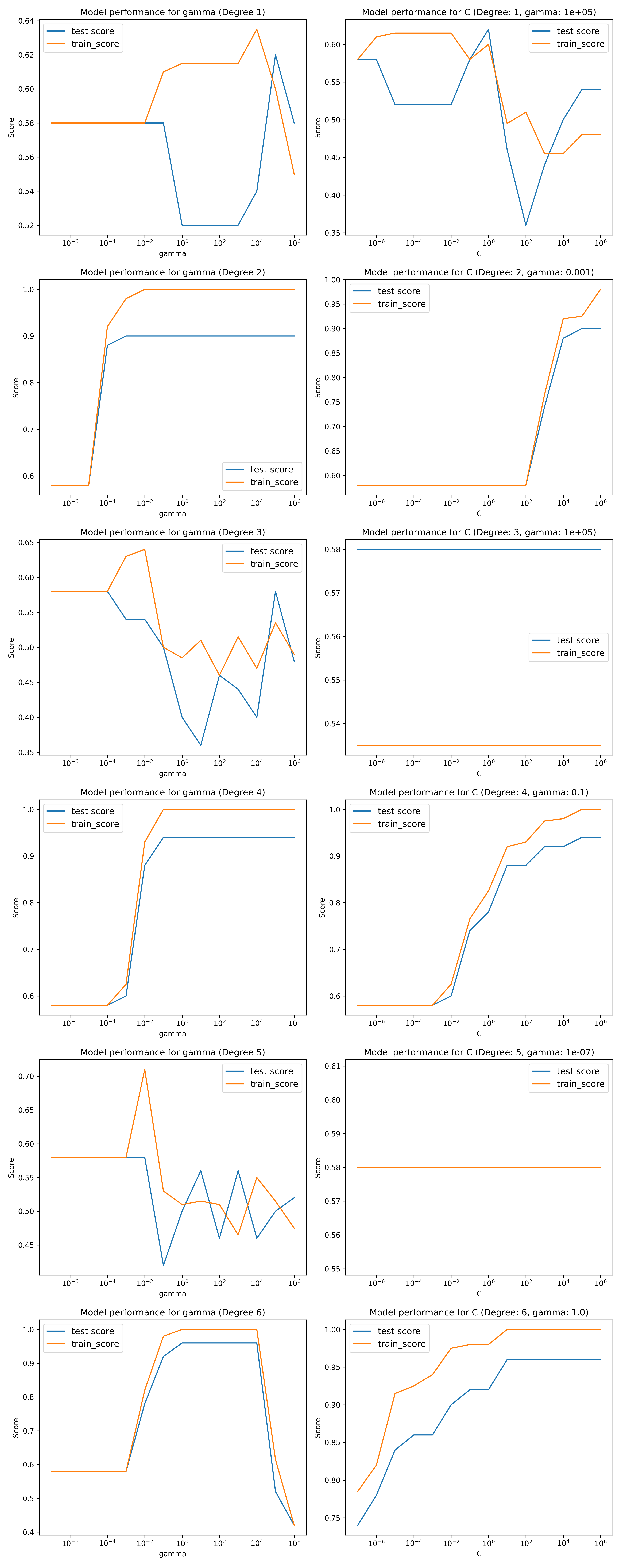
As you can see, the model perfoms better than the linear kernel but only for specific orders. The rows of the plot alternate depending on the order of the degree. The even degree polynomial fits score extremely well with test score in the 0.9-1 range for optimized cost and gamma values. This is to be expected as we are fitting quadratic functions, and polynomials of even degrees have similar shapes. However there is terrible performance for odd degrees, even as poorly as the linear model SVC. This is is due to the form of the odd degree polynomials. We had to limit the number of iterations on the fit as it took too long to fit an optimal solution to to the odd polynomial degrees.

Radial basis function kernel

We generate similar plots as the polynomial kernel. We use the follwoing code,

rbf_svm = SVC(kernel='rbf')
## Set the values to iterate over
### Gamma Values
# gamma_values = np.arange(0.001, 1, 0.01)
gamma_values = [np.power(10.0,x) for x in np.arange(-7,2,1)]
### Cost Values
# C_values = np.arange(0.001, 5, 0.01)
C_values = [np.power(10.0,x) for x in np.arange(-7,3,1)]

fig, (ax1, ax2) = plt.subplots(nrows=1, ncols=2, figsize=(12,6))
## Perform CV with gamma values
gamma_results = plot_score_vs_param(rbf_svm, X, y, para='gamma', param_values=gamma_values)
## Update model with best gamma value
rbf_svm.set_params(gamma=gamma_results['best_value'])
## Perform CV with C values
C_results = plot_score_vs_param(rbf_svm, X, y, para='C', param_values=C_values)

## Update axes with new plots
ax1.plot(gamma_values, gamma_results['test_scores'], label='test score')
ax1.plot(gamma_values, gamma_results['train_scores'], label='train_score')
ax1.set_xlabel('gamma')
ax1.set_ylabel('Score')
ax1.set_title('Model performance for gamma')
ax1.legend(fontsize = 'large')
ax1.set_xscale('log')

ax2.plot(C_values, C_results['test_scores'], label='test score')
ax2.plot(C_values, C_results['train_scores'], label='train_score')
ax2.set_xlabel('C')
ax2.set_ylabel('Score')
ax2.set_title('Model performance for C')
ax2.legend(fontsize = 'large')
ax2.set_xscale('log')

plt.tight_layout()
plt.savefig(os.path.join(IMAGE_DIR, 'q4_rbf_cv_plots.png'))
plt.show()
plt.close()

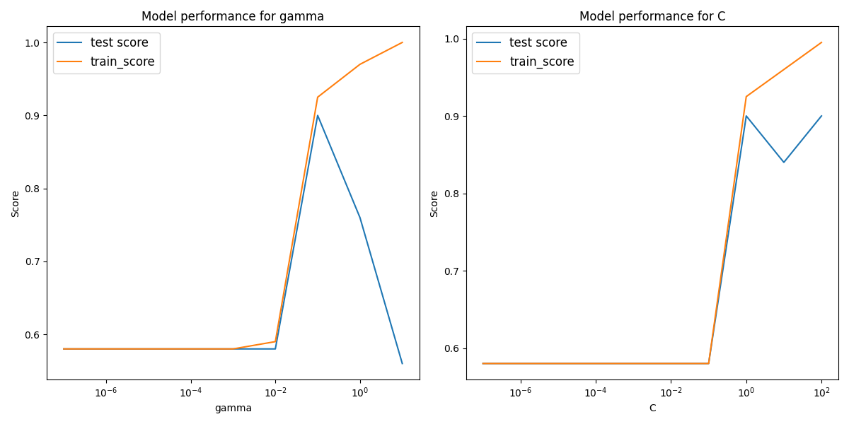
The rbf performs quite well on the plot which is expected as it is a very flexible model. It performs similar to the even degree polynomial SVCs, though here it is clear more hyperparamter optimization is needed than the polynomial fit as the performance does not follow a general trend in gamma or C.

PRSS Ridge

Problem Five

Part a)

Generate the predictors and classes with a linear decision boundary with,

## Set predictors and classes
x_1 = np.random.uniform(size=500) - 0.5
x_2 = np.random.uniform(size=500) - 0.5
X = np.column_stack((x_1, x_2))

y = []

for i in range(len(x_2)):
    arg = x_1[i]**2 - x_2[i]**2
    if arg > 0:
        y.append(1)
    else:
        y.append(-1)
y = np.array(y)

Part b)

Plot the data colored by classification

fig, ax = plt.subplots(1,1,figsize=(12,12))
sns.scatterplot(x=x_1, y=x_2, hue=y, ax=ax)

ax.set_xlabel('X_1')
ax.set_ylabel('X_2')
ax.set_title('Data set with quadratic decision boundary')

# plt.savefig(os.path.join(IMAGE_DIR,'q5_pb_class_plot.png'))
plt.show()
plt.close()

PRSS Ridge

Part c) and d)

Fit the normal logistic regression and plot the preditions of the training set,

## Instantiate the logistic regression model with the original predictors
logr = LogisticRegression()
## Fit the model
logr.fit(X,y)
## Predict the test set
y_preds = logr.predict(X)

## Plot the Predictions
fig, ax = plt.subplots(1,1,figsize=(12,12))
sns.scatterplot(x=X[:,0], y=X[:,1], hue=y_preds, ax =ax)

ax.set_xlabel('X_1')
ax.set_ylabel('X_2')
ax.set_title('Predicted class set with vanilla Logistic Regression')

# plt.savefig(os.path.join(IMAGE_DIR,'q5_pcd_class_plot.png'))
plt.show()
plt.close()

PRSS Ridge

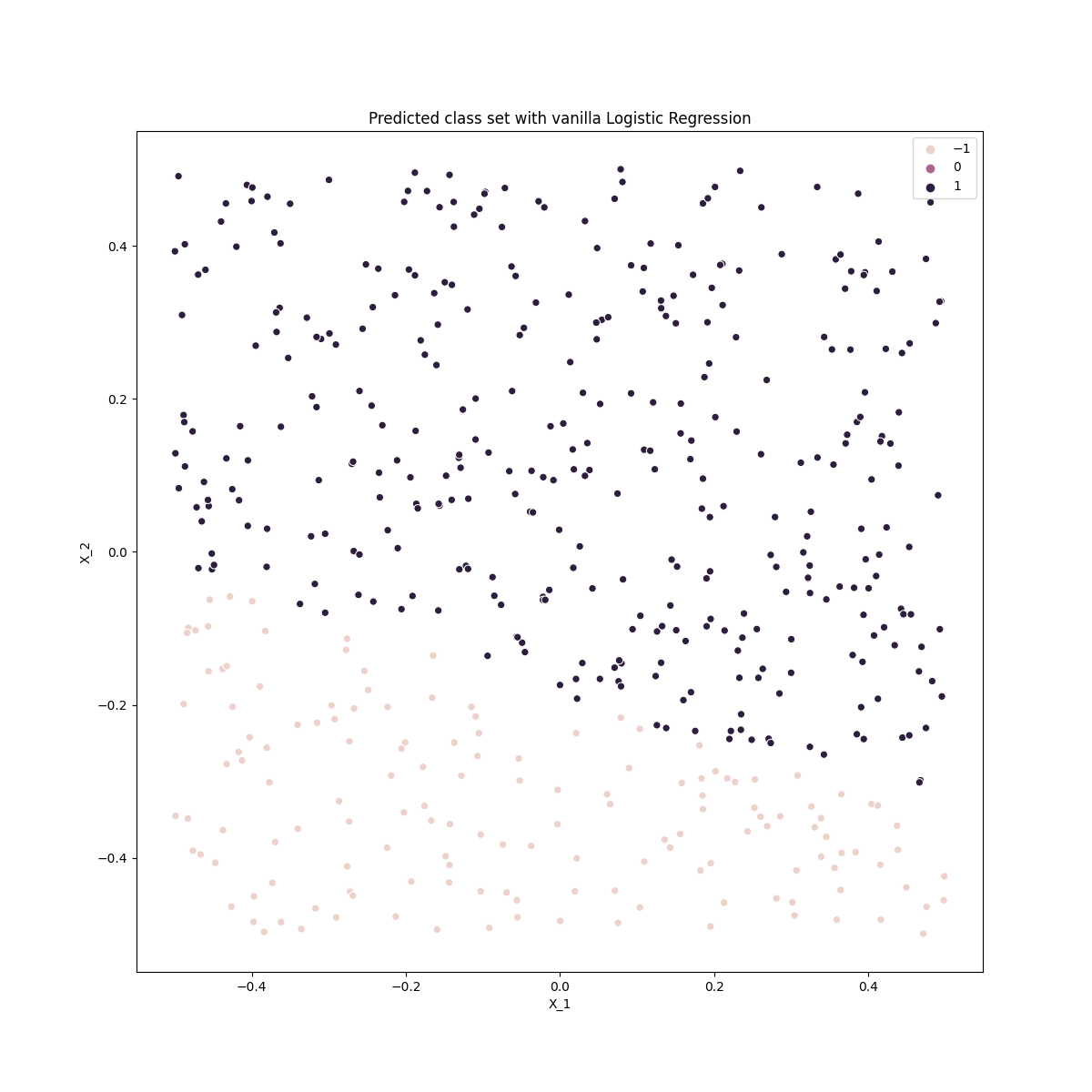
This is clearly a poor classifier as classifies a linear decision boundary as expected

Part e) and f)

## Preprocessing
x_12 = np.multiply(X[:,0], X[:,1]).reshape(X.shape[0], 1)
x_1_squared = np.multiply(X[:,0], X[:,0]).reshape(X.shape[0], 1)
x_2_squared = np.multiply(X[:,1], X[:,1]).reshape(X.shape[0], 1)

extra_pred_list = [x_12, x_1_squared, x_2_squared]

for arr in extra_pred_list:
    X = np.append(X, arr, axis=1)

logr = LogisticRegression()
logr.fit(X,y)
y_preds = logr.predict(X)

fig, ax = plt.subplots(1,1,figsize=(12,12))
sns.scatterplot(x=X[:,0], y=X[:,1], hue=y_preds, ax =ax)

ax.set_xlabel('X_1')
ax.set_ylabel('X_2')
ax.set_title('Predicted class set with feature expanded Logistic Regression')

# plt.savefig(os.path.join(IMAGE_DIR,'q5_pef_class_plot.png'))
plt.show()
plt.close()

PRSS Ridge

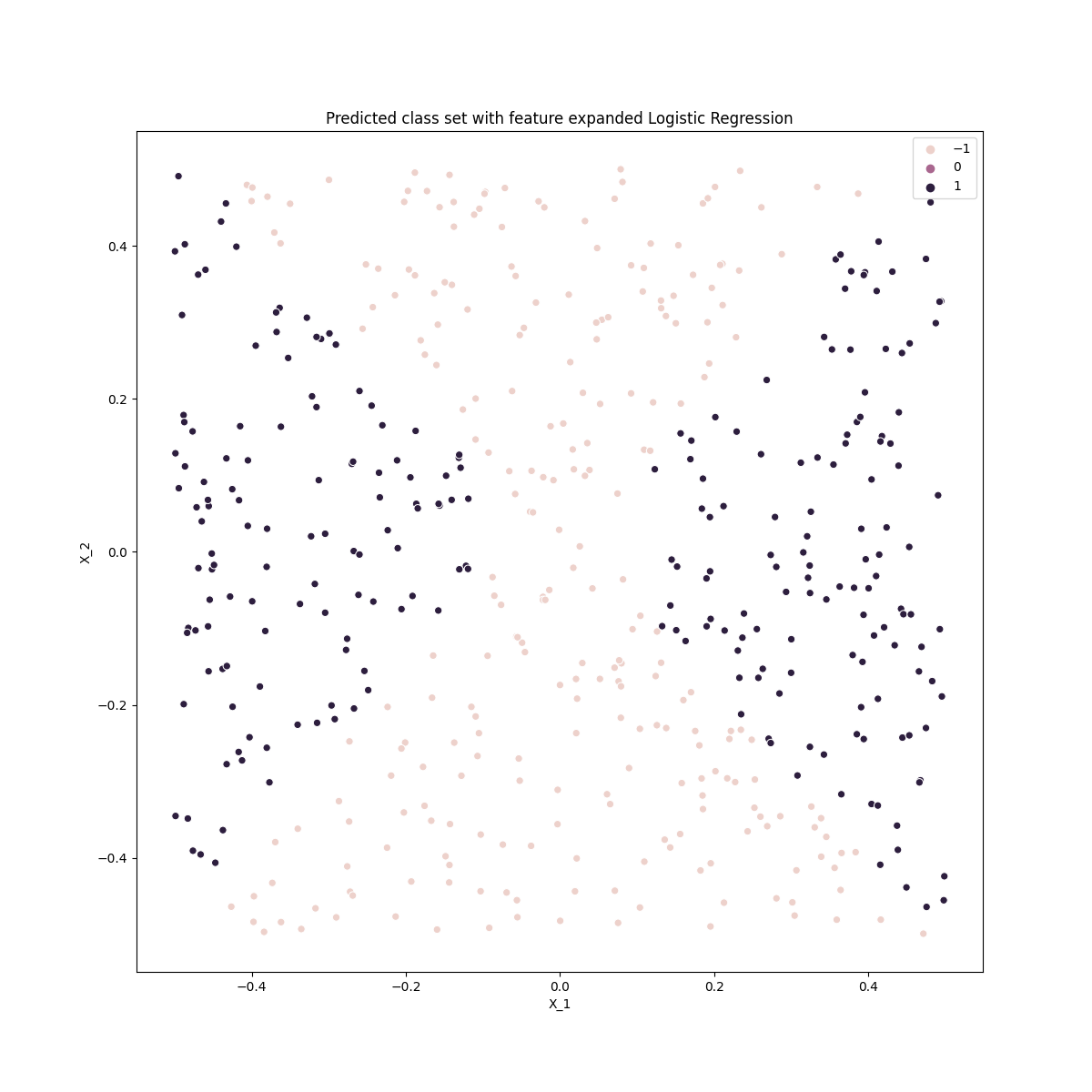
Comparing this with the original data we can see that the logistic classifier with an expanded feature space dreproduces the quadratic decision boundaries.

Part g)

lin_svc = SVC(kernel='linear', C=10)
lin_svc.fit(X,y)
y_preds = lin_svc.predict(X)

fig, ax = plt.subplots(1,1,figsize=(12,12))
sns.scatterplot(x=X[:,0], y=X[:,1], hue=y_preds, ax =ax)

ax.set_xlabel('X_1')
ax.set_ylabel('X_2')
ax.set_title('Predicted class set with linear SVC')

plt.savefig(os.path.join(IMAGE_DIR,'q5_pg_class_plot.png'))
# plt.show()
plt.close()

PRSS Ridge

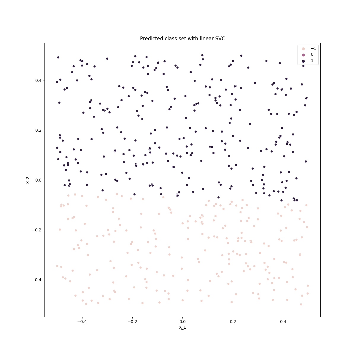
The linear SVC performs similarly to the logistric classification with only the orginal features.

Part h)

poly_svc = SVC(kernel='poly', C=10, degree=2)
poly_svc.fit(X,y)
y_preds = poly_svc.predict(X)

fig, ax = plt.subplots(1,1,figsize=(12,12))
sns.scatterplot(x=X[:,0], y=X[:,1], hue=y_preds, ax =ax)

ax.set_xlabel('X_1')
ax.set_ylabel('X_2')
ax.set_title('Predicted class set with quadratic SVC')

plt.savefig(os.path.join(IMAGE_DIR,'q5_ph_class_plot.png'))
# plt.show()
plt.close()

PRSS Ridge

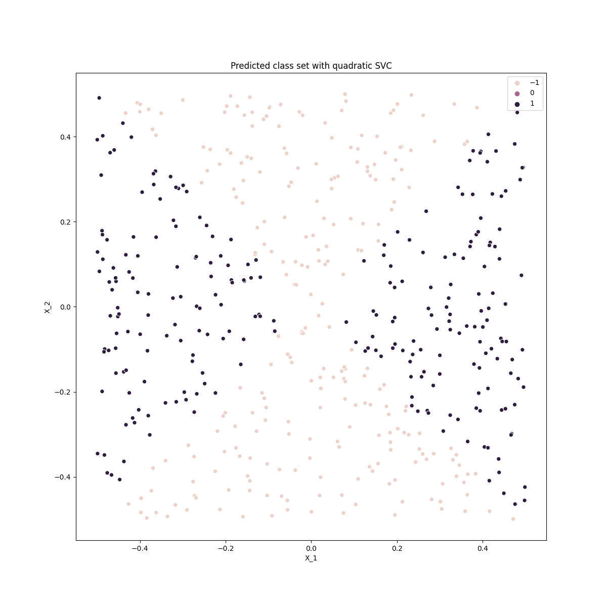
The polynomial SVC (of degree 2) performs well, similar to the logistic regression with expanded feature space. Note that here the polynomial degree must be even (see problem 4) otherwise it has similarly poor performance as the linear model.

Problem Seven

Part a)

Load the auto dataset and create the classification column based on the median mpg,

## Load the auto dataset
auto_df = pd.read_csv(os.path.join(DATA_DIR, 'auto.csv'))
## Create the classification column based on the median mpg
median_mpg = auto_df['mpg'].describe()['50%']
auto_df['mpg01'] = auto_df['mpg'].apply(lambda x: 1 if x > median_mpg else 0)
## Clean up remaining data
auto_df = auto_df[auto_df['horsepower'] != '?']
auto_df['horsepower'] = auto_df['horsepower'].apply(lambda x: float(x))

Part b)

Find the best performance of the linear model with cross-validation (we use the same function plot_score_vs_param defined in problem four),

## Instantiate the linear SVC
linear_svm = SVC(kernel='linear')
C_values = [np.power(10.0,x) for x in np.arange(-7,7,1)]

C_results = plot_score_vs_param(linear_svm , X, y, para='C', param_values=C_values)

fig, ax1 = plt.subplots(nrows=1, ncols=1, figsize=(12,6))
ax1.plot(C_values, C_results['test_scores'], label='test score')
ax1.plot(C_values, C_results['train_scores'], label='train_score')

ax1.set_xlabel('C')
ax1.set_ylabel('Score')
ax1.set_title('Model performance for C')
ax1.legend(fontsize = 'large')
ax1.set_xscale('log')

# plt.savefig(os.path.join(IMAGE_DIR, 'q7_linear_C_plot.png'))
plt.show()
plt.close()

Best value of cost (C):  10.0
Best test set score:  0.995

Produces the plot,

PRSS Ridge

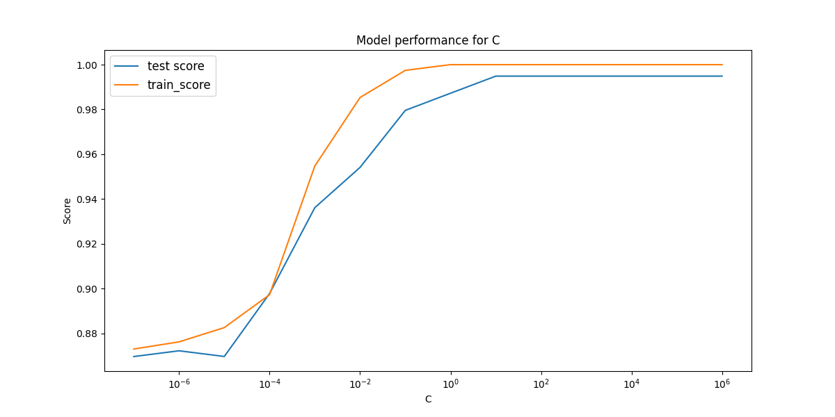
This linear model performs incredibly we considering the test score of 0.995!

Part c)

We now do similar approachs with the polynomial and rbf kernels. Here we use near identical code that of problem 4 to produce the hyperparameter plots.

Polynomial kernel

The polynomial hyper-parameter plots are,

PRSS Ridge

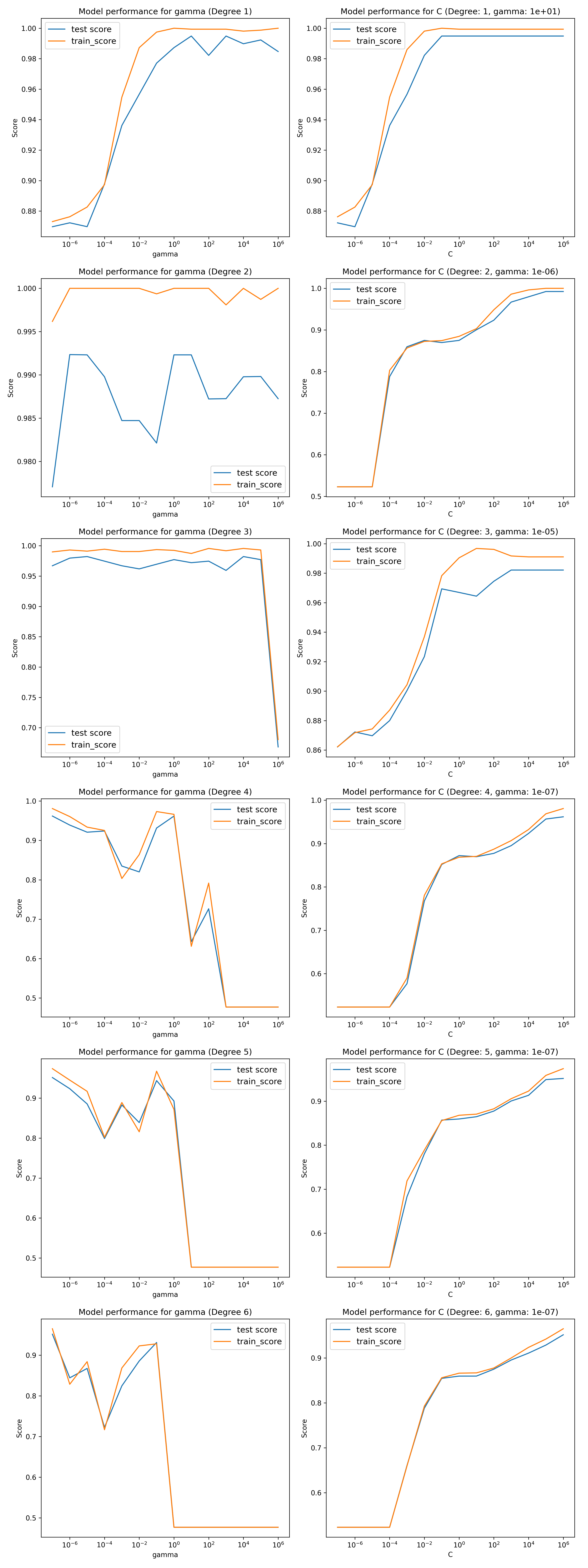
Once again, the cost and gamma hyper-parameters are not independent and there may be some combinations of them which give better performance than presented. Though this is a naive approach, it is sufficient to demonstrate the model performance.

Here we see that for all degrees, there is a combination of hyper-parameters that performs very well, better than the linear model (degree=1 is the linear model with different hyperparameters). They all have an optimized training score of close to 1.

It is interesting to note the difference between these results and those of the polynomial fit in Problem four. In problem 4 the odd degreee polynomials had poor fits and the even very good fits where here all degrees have very good fits. This is because i the problem 4 dataset there were only two predictors with a fixed quadratic boundary. In this dataset there are many predictors and therefore the possible number of good boundary of different degrees is very large.

RBF kernel

The RBF hyperparameter plots are below,

PRSS Ridge

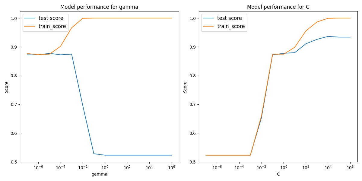
We see here that the rbf kernel did not perform as well as either the polynomial or linear SVCs.

Chapters

Basics

Regression

Classification

Resampling

Regularization

Beyond Linearity

Tree Models

Support Vector Machines

Unsupervised Learning

Contents

Chapter Nine: Support Vector Machines

Applied Problems

Problem Four

Linear kernel

Polynomial kernel

Radial basis function kernel

Problem Five

Part a)

Part b)

Part c) and d)

Part e) and f)

Part g)

Part h)

Problem Seven

Part a)

Part b)

Part c)

Polynomial kernel

RBF kernel