Chapter Eight: Tree-Based Models

Applied Problems

Load all the standard modules

import pandas as pd
import numpy as np
import os

import matplotlib.pyplot as plt
import seaborn as sns

np.random.seed(101)

Problem Seven

Load in the dataframe and separete the target and predictors.

boston_df = pd.read_csv(os.path.join(DATA_DIR, "boston.csv"))
X = boston_df.drop('target', axis=1)
y = boston_df['target']

Instantiate the random forest regressor

from sklearn.ensemble import RandomForestRegressor
f_model = RandomForestRegressor()

Number of features considered

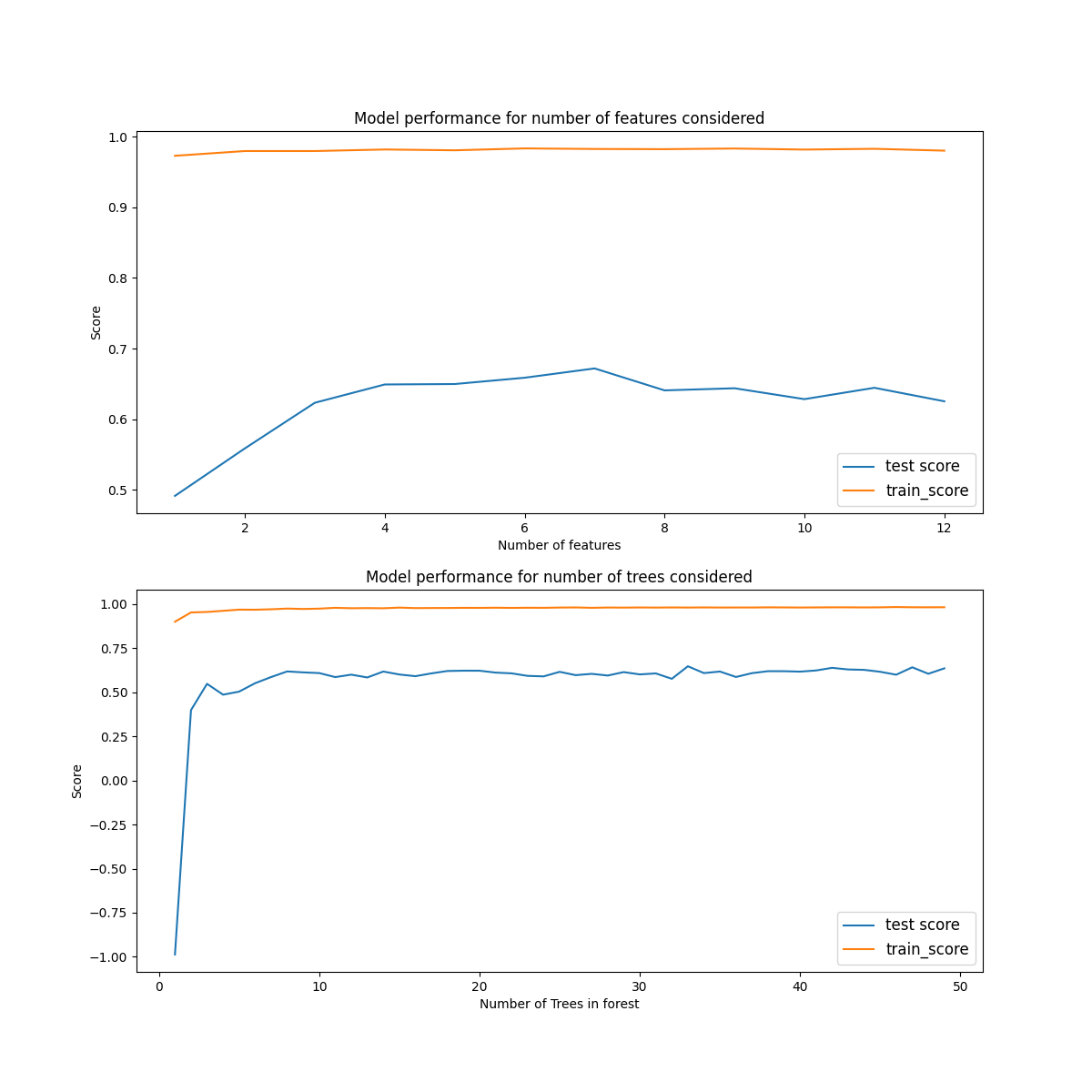
We will first find the ideal maximium number of predictors to consider at each split. In sklearn this is controller by the max_features variable. We iterate over this in a for loop, cross-validating the model and storing the training and testing errors in a list. The scores are standard $R^2$ values.

from sklearn.model_selection import cross_validate
## Create an array of integers to iterate over
num_feats = np.arange(1,X.shape[1])
## Set the number of trees to be constant.
f_model.set_params(n_estimators=50)
## Create empty lists for training and testing scores
test_cv_scores_feats = []
train_cv_scores_feats = []
## Loop over the number of features
for i in num_feats:
    print(i)
    ## Update the regressor and cross_validate
    f_model.set_params(max_features = i)
    scores = cross_validate(f_model, X, y, return_train_score=True)
    test_cv_scores_feats.append(scores['test_score'].mean())
    train_cv_scores_feats.append(scores['train_score'].mean())

The results are plotted in the figure below. We can see that the training score consistently performs very well, even when considering only 1 feature. However the training set is affected quite significantly with maximum performance of $R^2_{test} \approx 0.7$ for 7 features considered. In this model we have fixed the number of trees at $50$, there may be different outcomes for the models dependence if a different value was used.

Number of trees used in the forest

Next we will study how the number of decision trees used in aggregating the forest affects its performance.

## Create an array of integers to iterate over
num_trees = np.arange(1,50,1)
## Set the number of predictors considered at each step to be constant. In this case we use the total number of predictors
f_model.set_params(max_features = X.shape[1])
## Create empty lists for training and testing scores
test_cv_scores_ntrees = []
train_cv_scores_ntrees = []
## Loop over the number of trees
for trees in num_trees:
    print(trees)
    f_model.set_params(n_estimators = trees)
    scores = cross_validate(f_model, X, y, return_train_score=True)
    test_cv_scores_ntrees.append(scores['test_score'].mean())
    train_cv_scores_ntrees.append(scores['train_score'].mean())

The results are plotted in the figure below.

Here again the training score performs extremely well for all tree numbers considered. The test score starts off poorly but quite reaches uniformity for N-trees=4 and does not significantly change after that. However, this test score is quite poor at $R^2 \approx 60$.

Problem Eight

Load the carseat data and preprocess it for modeling by one-hot encoding the categorical variables,

## Load dataframe
carseats_df = pd.read_csv(os.path.join(DATA_DIR, "carseats.csv"))
carseats_df.set_index('Unnamed: 0', inplace=True)
print(carseats_df.info())

##Preprocessing
carseats_df = pd.get_dummies(carseats_df,['Urban', 'US', 'ShelveLoc'], drop_first=True)

y = carseats_df['Sales']
X = carseats_df.drop('Sales', axis=1)

Part a)

Split the data into training and test sets,

from sklearn.model_selection import train_test_split
## Split in test and training sets
X_train, X_test, y_train, y_test = train_test_split(X, y, random_state=42)

Part b)

Create a model with a single decision tree and find its test and training scores,

from sklearn.tree import DecisionTreeRegressor
## Instantiate the decision tree
tree = DecisionTreeRegressor()
## FIt the tree
tree.fit(X_train, y_train)
## Score the tree
score = tree.score(X_test, y_test)
print('Test score: ', round(score,2))
score = tree.score(X_train, y_train)
print('Train score: ', round(score,2))

Test score:  0.44
Train score:  1.0

Part c)

## Instantiate the decision tree
tree = DecisionTreeRegressor()

## Create set of test alpha values and empty cv scores for training and testing
alpha_value = np.arange(0,1, 0.001)
cv_score_alpha_test = []
cv_score_alpha_train = []

## iterate of alpha and score the training and test results
for a in alpha_value:
    print(a)
    tree.set_params(ccp_alpha = a)
    scores = cross_validate(tree, X, y, return_train_score=True)
    cv_score_alpha_test.append(scores['test_score'].mean())
    cv_score_alpha_train.append(scores['train_score'].mean())

## Plot the training and test scores
fig, ax = plt.subplots(1,1,figsize=(12,6))
ax.plot(alpha_value, cv_score_alpha_test, label = 'test score')
ax.plot(alpha_value, cv_score_alpha_train, label = 'training score')

ax.set_xlabel(r'\alpha', fontsize = 'large')
ax.set_ylabel('Score (R -squared)', fontsize = 'large')
ax.set_title('Model performance as pruning is increased', fontsize = 'xx-large')
ax.legend(fontsize = 'large')

# plt.savefig(os.path.join(IMAGE_DIR, 'q8_tree_complexity_plot.png'))
plt.show()
plt.close()

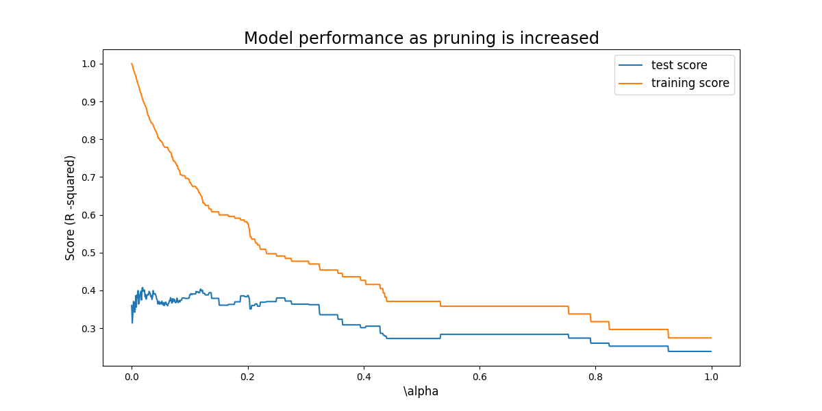
Considering just this simple tree pruning does not have a positive affect on the test error. As we expect, the training score decreases as the comlexity is reduced, however this does not result in the increase in test score (other than a small amount) we hope for.

Part d)

Employ a bagging approach,

from sklearn.ensemble import BaggingRegressor
## Store a list of column names
cols = X.columns
## Instaniate the regressor
tree = DecisionTreeRegressor()
## Instantiate and fit the bagger
bagger = BaggingRegressor(base_estimator=tree)
bagger.fit(X_train,y_train)

## Score the test set with the bagger
print('Test Score: ', bagger.score(X_test, y_test))

## Create a dictionary of feature importances in the modeal and sort them
feat_import = bagger.estimators_[0].feature_importances_
feat_import = dict(zip(cols, feat_import))
feat_import = {k: v for k, v in sorted(feat_import.items(), key=lambda item: item[1], reverse = True)}
for key, val in feat_import.items():
    print("{0:<20} : {1:<20}".format(key, round(val,3)))

Test Score:  0.665801010524065
Price                : 0.336
Urban_Good           : 0.2
CompPrice            : 0.109
Income               : 0.094
Urban_Medium         : 0.084
Age                  : 0.057
Advertising          : 0.05
Population           : 0.039
Education            : 0.025
US_Yes               : 0.005
ShelveLoc_Yes        : 0.0

Here price is the most important predictor of sales (as expected).

Part e)

Very similar approach as the bagging model above,

cols = X.columns
## Instantiate the decision tree
forest = RandomForestRegressor()
## Fit the tree
forest.fit(X_train, y_train)
## Score the tree
score_R2 = forest.score(X_test, y_test)
print('Test score (R-squared): ', round(score_R2,2))

preds = forest.predict(X_test)

score_MSE = mean_squared_error(y_test, preds)
print('Test score (MSE): ', round(score_MSE,2))

feat_import = forest.feature_importances_
feat_import = dict(zip(cols, feat_import))
## Sort by feature_importance
feat_import = {k: v for k, v in sorted(feat_import.items(), key=lambda item: item[1])}
for key, val in feat_import.items():
    print("{0:<20} : {1:<20}".format(key, round(val,3)))

Test score (R-squared):  0.7
Test score (MSE):  2.79
Price                : 0.321
Urban_Good           : 0.199
Age                  : 0.11
CompPrice            : 0.1
Advertising          : 0.084
Urban_Medium         : 0.055
Income               : 0.046
Population           : 0.041
Education            : 0.031
US_Yes               : 0.007
ShelveLoc_Yes        : 0.006

Problem Nine

Load the dataset

## Load dataframe
oj_df = pd.read_csv(os.path.join(DATA_DIR, "OJ.csv"))
y = oj_df['Purchase']
X = oj_df.drop(['Purchase', 'Store7'], axis=1)

Part a)

X_train, X_test, y_train, y_test = train_test_split(X, y, test_size=800)
## Instantiate the decission tree classifier
tree = DecisionTreeClassifier()

## Fit the tree to the training data
tree.fit(X_train, y_train)
## Score the training and test set
test_score = tree.score(X_test,y_test)
train_score = tree.score(X_train, y_train)
## Print properties of the tree
depth = tree.get_depth()
num_leaves= tree.get_n_leaves()

print('test score: ', round(test_score,2))
print('train score: ', round(train_score,2))
print('tree depth: ', depth)
print('terminal nodes (leaves): ', num_leaves)

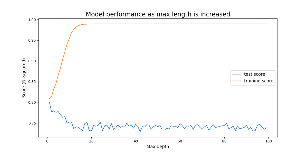
test score:  0.74
train score:  0.99
tree depth:  11
terminal nodes (leaves):  67

Part e)

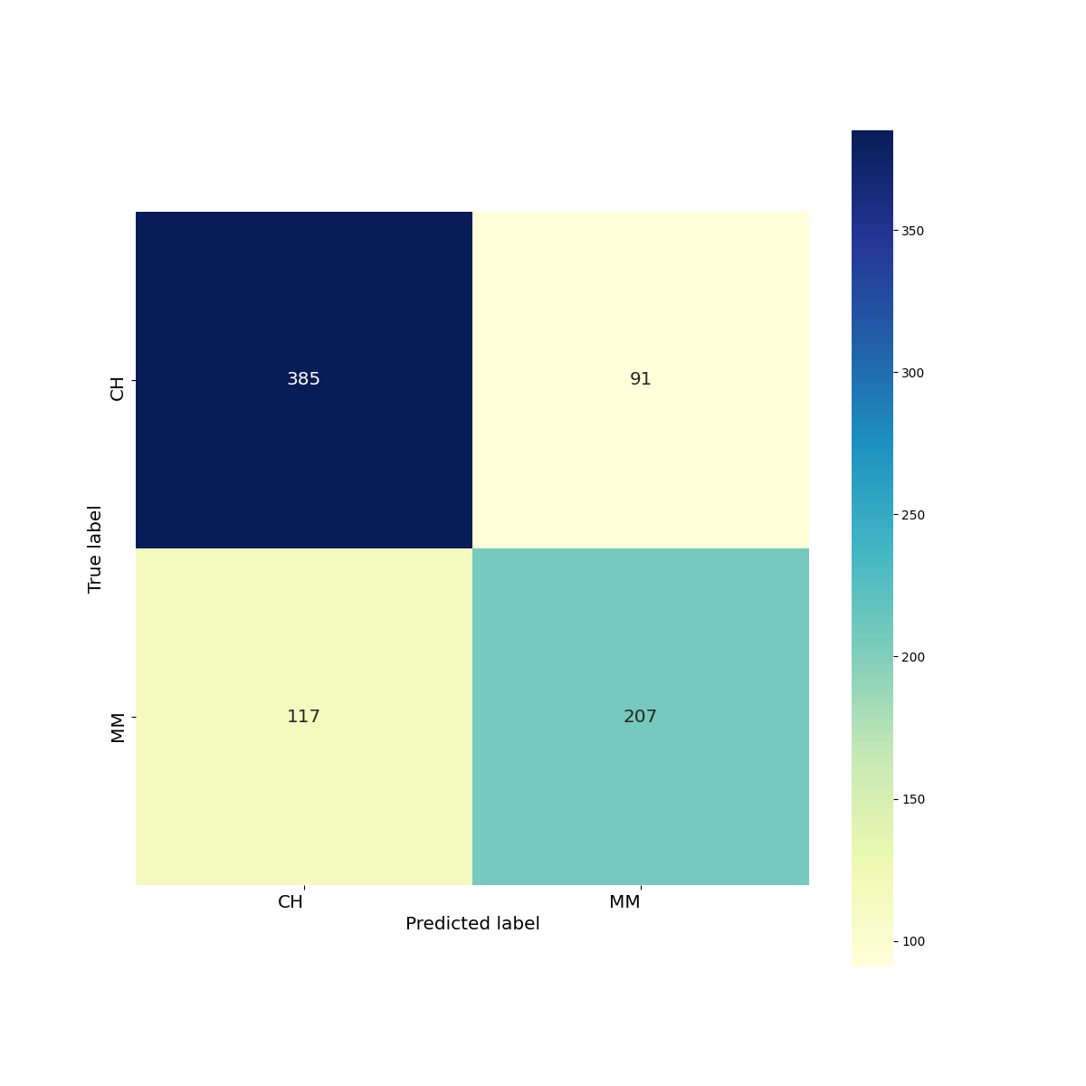
The confusion matrix is,

## Split the training and test set
X_train, X_test, y_train, y_test = train_test_split(X, y, test_size=800)

## Instantiaate the model
tree = DecisionTreeClassifier()

## Fit and predict the model
tree.fit(X_train, y_train)
preds = tree.predict(X_test)
## Generate the confusion_matrix
cm = confusion_matrix(y_test, preds, labels=['CH', 'MM'])
# unique, counts = np.unique(y_test, return_counts=True)
# print('true counts: ', dict(zip(unique, counts)))
# unique, counts = np.unique(preds, return_counts=True)
# print('pred counts: ', dict(zip(unique, counts)))
# print(cm)

## Plot the confusion matrix
fig, ax = plt.subplots(1,1, figsize=(12,12))
heatmap = sns.heatmap(cm, annot=True, fmt='d', cmap="YlGnBu", xticklabels = ['CH', 'MM'], yticklabels=['CH', 'MM'], annot_kws={'fontsize':'x-large'}, ax=ax, square=True)
heatmap.yaxis.set_ticklabels(heatmap.yaxis.get_ticklabels(), ha='right', fontsize='x-large')
heatmap.xaxis.set_ticklabels(heatmap.xaxis.get_ticklabels(), ha='right', fontsize='x-large')
ax.set_ylabel('True label', fontsize='x-large')
ax.set_xlabel('Predicted label', fontsize='x-large')
plt.savefig('q9_cm_heatmap.png')
plt.show()

print(classification_report(y_test, preds))

                   precision    recall  f1-score   support

CH                 0.77      0.81      0.79       476
MM                 0.69      0.64      0.67       324

accuracy                               0.74       800
macro avg          0.73      0.72      0.73       800
weighted avg       0.74      0.74      0.74       800

Part g)

## Instantiate the decision tree
tree = DecisionTreeClassifier()
best_score=0

## Create set of test alpha values and empty cv scores for training and testing
max_size_value = np.arange(1,100)
cv_score_depth_test = []
cv_score_depth_train = []

## iteracte of alpha and score the training and test results
for l in max_size_value:
    print(l)
    tree.set_params(max_depth = l)
    scores = cross_validate(tree, X, y, return_train_score=True, return_estimator=True)
    cv_score_depth_test.append(scores['test_score'].mean())
    cv_score_depth_train.append(scores['train_score'].mean())


## Plot the training and test scores
fig, ax = plt.subplots(1,1,figsize=(12,6))
ax.plot(max_size_value, cv_score_depth_test, label = 'test score')
ax.plot(max_size_value, cv_score_depth_train, label = 'training score')

ax.set_xlabel(r'Max depth', fontsize = 'large')
ax.set_ylabel('Score (R -squared)', fontsize = 'large')
ax.set_title('Model performance as max length is increased', fontsize = 'xx-large')
ax.legend(fontsize = 'large')

plt.savefig(os.path.join(IMAGE_DIR, 'q9_tree_depth_plot.png'))
plt.show()
plt.close()

Problem Ten

Load the data and preprocess the data by removing invalid entries, on-hot encoding the categorical variables and log transforming the Salary variable.

Part a)

## Load dataframe
hitters_df = pd.read_csv(os.path.join(DATA_DIR, "Hitters.csv"))
print('columns: ', list(hitters_df.columns))
# print(hitters_df.info())

## Drop the rows where salary is NaN
hitters_df.dropna(subset=['Salary'], inplace=True)

## Log transform Salary
hitters_df['log_Salary'] = hitters_df['Salary'].apply(lambda x: np.log(x))

## One-hot encode the object columns
hitters_df = pd.get_dummies(hitters_df, ['League', 'Division', 'NewLeague'], drop_first=True)

y = hitters_df['log_Salary']
X = hitters_df.drop(['Salary', 'log_Salary'], axis=1)

Part b)

X_train, X_test, y_train, y_test = train_test_split(X, y, train_size=200)

Part c)

alpha_values = np.arange(0, 10, 0.001)
lambda_values = np.arange(0, 10, 0.001)
# alpha_values = [np.power(10.0,x) for x in np.arange(-10,1,1)]
# lambda_values = [np.power(10.0,x) for x in np.arange(-10,1,1)]
cv_score_alpha_test = []
cv_score_alpha_train = []
cv_score_lambda_test = []
cv_score_lambda_train = []

boost = xgb.XGBRegressor(n_estimators=1000, objective='reg:squarederror')

# boost.fit(X,y)
# preds = boost.predict(X)
# print(preds)

boost.set_params(reg_lambda=0)

for alpha in alpha_values:
    print(alpha)
    boost.set_params(reg_alpha=alpha)
    scores = cross_validate(boost, X, y, return_train_score=True, n_jobs=-1)
    print(scores['test_score'].mean())
    print(scores['train_score'].mean())
    cv_score_alpha_test.append(scores['test_score'].mean())
    cv_score_alpha_train.append(scores['train_score'].mean())

boost.set_params(reg_alpha=0)

for lam in lambda_values:
    print(lam)
    boost.set_params(reg_lambda=lam)
    scores = cross_validate(boost, X, y, return_train_score=True, n_jobs=-1)
    print(scores['test_score'].mean())
    print(scores['train_score'].mean())
    cv_score_lambda_test.append(scores['test_score'].mean())
    cv_score_lambda_train.append(scores['train_score'].mean())

## Plot the results of each cv loop. Both training and testing.
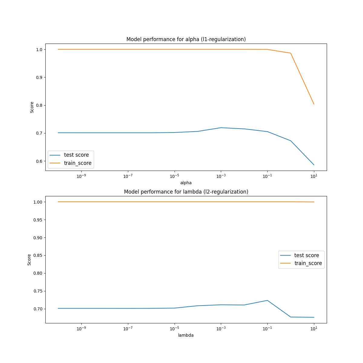
fig, ((ax1), (ax2)) = plt.subplots(nrows=2, ncols=1, figsize=(12,12))
ax1.plot(alpha_values, cv_score_alpha_test, label='test score')
ax1.plot(alpha_values, cv_score_alpha_train, label='train_score')

ax2.plot(lambda_values, cv_score_lambda_test, label='test score')
ax2.plot(lambda_values, cv_score_lambda_train, label='train_score')

ax1.set_xlabel('alpha')
ax1.set_ylabel('Score')
ax1.set_title('Model performance for alpha (l1-regularization)')
ax1.legend(fontsize = 'large')

ax2.set_xlabel('lambda')
ax2.set_ylabel('Score')
ax2.set_title('Model performance for lambda (l2-regularization)')
ax2.legend(fontsize = 'large')

plt.savefig(os.path.join(IMAGE_DIR, 'q10_regularization_performance.png'))
plt.show()

Part d)

We check use a similar iterative loop to find the shrinkge values as we did with the regularization parameters in part c). First we do an order of magnitude plot to see how it changes for large values.

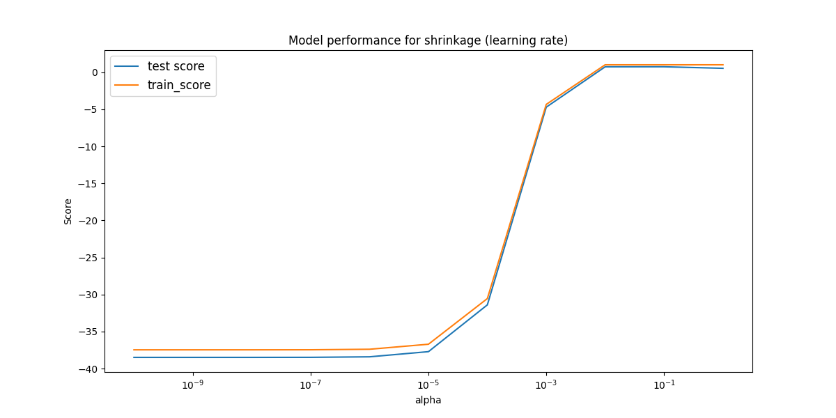
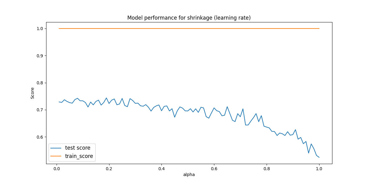
Here there is only reasonable performance between 0.01 and 1. Therefore, we check that region in paricular to see if there are any peaks.

Problem Eleven

## Load dataframe
caravan_df = pd.read_csv(os.path.join(DATA_DIR, "caravan.csv"))

y = caravan_df['Purchase']
X = caravan_df.drop('Purchase', axis=1)
X_cols = X.columns

Part a)

X_train, X_test, y_train, y_test = train_test_split(X, y, train_size=1000, random_state=101)

Part b)

Find the test score with xgboost classifier and find the top 5 important features.

X_cols = X.columns
X_train, X_test, y_train, y_test = train_test_split(X, y, train_size=1000, random_state=101)

boost = xgb.XGBClassifier(n_estimators=1000, reg_alpha=0.01, random_state=101)
boost.fit(X_train,y_train)
print('test set score: ', boost.score(X_test, y_test))

feat_import = list(zip(X_cols, boost.feature_importances_))
feat_import.sort(key=lambda tup: tup[1], reverse=True)
for feat in feat_import[0:5]:
    print("{0:<20}:{1:<20}".format(feat[0], feat[1]))

test set score:  0.921401907922024
PFIETS              :0.17959140241146088
MINK123M            :0.03962616249918938
MGODOV              :0.037652637809515
MBERHOOG            :0.03663846105337143
MBERBOER            :0.03459399193525314

Part c)

X_train, X_test, y_train, y_test = train_test_split(X, y, train_size=1000, random_state=101)

boost = xgb.XGBClassifier(n_estimators=1000, reg_alpha=0.01, random_state=101)
boost.fit(X_train,y_train)
boost_prob_preds = boost.predict_proba(X_test)

knn = KNeighborsClassifier()
knn.fit(X_train, y_train)
knn_prob_preds = knn.predict_proba(X_test)

logr = LogisticRegression()
logr.fit(X_train, y_train)
logr_prob_preds = logr.predict_proba(X_test)

threshold = 0.2

threshold_v = np.vectorize(lambda x: 'No' if x < threshold else 'Yes')
boost_prob_preds = threshold_v(boost_prob_preds[:,1])
knn_prob_preds = threshold_v(knn_prob_preds[:,1])
logr_prob_preds = threshold_v(logr_prob_preds[:,1])

boost_cm = confusion_matrix(y_test.values, boost_prob_preds)
knn_cm = confusion_matrix(y_test.values, knn_prob_preds)
logr_cm = confusion_matrix(y_test.values, logr_prob_preds)

fig, ((ax1), (ax2), (ax3)) = plt.subplots(nrows=3, ncols=1)
sns.heatmap(boost_cm, annot=True, fmt="d", ax = ax1) #annot=True to annotate cells
sns.heatmap(knn_cm, annot=True, fmt="d", ax = ax2)
sns.heatmap(logr_cm, annot=True, fmt="d", ax = ax3)

# labels, title and ticks
ax1.set_xlabel('Predicted labels')
ax1.set_ylabel('True labels')
ax1.set_title('XGBoost Confusion Matrix')
ax1.xaxis.set_ticklabels(['No', 'Yes'])
ax1.yaxis.set_ticklabels(['No', 'Yes'])

ax2.set_xlabel('Predicted labels')
ax2.set_ylabel('True labels')
ax2.set_title('KNN Confusion Matrix (N=5)')
ax2.xaxis.set_ticklabels(['No', 'Yes'])
ax2.yaxis.set_ticklabels(['No', 'Yes'])

ax3.set_xlabel('Predicted labels')
ax3.set_ylabel('True labels')
ax3.set_title('Logistic Regression Confusion Matrix')
ax3.xaxis.set_ticklabels(['No', 'Yes'])
ax3.yaxis.set_ticklabels(['No', 'Yes'])

fig.suptitle('Classifier Confusion Matricies for 20% threshold')

plt.savefig('q11_confusion_matrices.png')
plt.show()

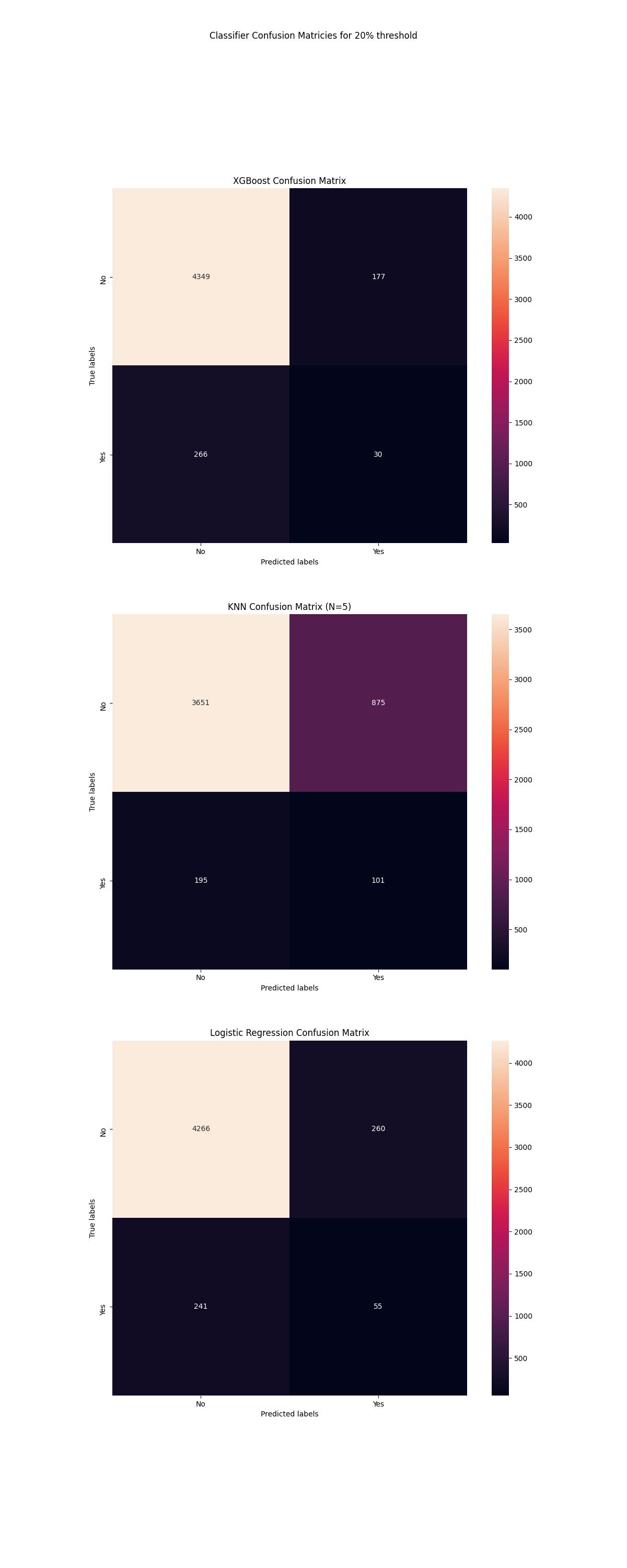
The worst classifier of these models is the KNN classifier, however it has not been optimized for the number of neighbours so that should be considered. The logistic regression model and xgboost model have similar performances at a glance. In a direct accuracy measure, the XGBoost performs slightly better. XGboost reported fewer false postives which is an important metric for many applications.