Thompson sampling with Non-Contextual bandits
The case of non-contextual bandits are much simpler than when contextual features are involved. We will consider a binary bandit where there is an underlying probability ($p_i$) of the $i$th arm either paying out a reward ($r=1$) or not ($r=0$).
Background
Thompson sampling is a bayesian approach to reinforcement learning. Starting from informed priors for the underlying parameters governing the bandit, we explore by sampling the priors of each arm, selecting the highest value and pulling it.
Each arm has a binary probability $p_i$ of reward and therefore the reward can modeled as a Bernoulli distribution. The probability random variables themselves are confined to the range [0,1] and can be modeled as Beta distributions.
\begin{align} r_i \sim Bernoulli(p_i) \\ p_i \sim Beta(a_i, b_i) \end{align}
where $a_i$ and $b_i$ are the parameters which control the shape of the distribution.
Analytical approach
The simplicity of this setup is that we can use the conception of conjugative bayesian pairs. That is, the functional form of the posterior is the same as the prior given a specific likelihood function.
Updating the probability distribution
Using the conjugate pair concept of the beta distribution and Bayes theorem we can continuously update the probability of success by just tracking the number of attempts and number of successes. Starting from a completely uniformed uniform prior ($Beta(a=1, b=1)$) the poterior probability after $n$ attempts and $s$ successes is ($Beta(a'=s+1, b'=n-s+1)$). For a completely fair coin ($p=0.5$) $a'\approx b'$ and the beta distribution will be centered around $p=0.5$ and become narrower the more attempts (evidence) there are.
To demonstrate this, we can set up a bandit with just a single arm. In this case the agent does not need to sample and choose between the arms, but will learn and update its statistics on the single arm.
Import the required packages.
import tensorflow_probability as tfp
import tensorflow as tf
import pandas as pd
import numpy as np

tfd = tfp.distributions

print(tfp.__version__)
Set up a bernoulli distribution as out binary arm to draw our rewards from. We will use an 80% payout probability.
def pull_arm(p=0.8):
    reward = tfd.Bernoulli(
            probs=p,
            dtype=tf.float32,
            name='Bernoulli'
        ).sample().numpy()
    return reward
The 'agent' here will just be a list which stores the number of attempts (0) in the and the number of successes (1). Since there is no choice required, there only needs to be an action function.
hist = [0, 0]
def agent_action():
    reward = pull_arm()
    hist[0] += 1
    if reward == 1:
        hist[1] += 1
Assuming that our agent knows nothing about the probabiliity at the start, it has a completely uniformed prior on the probability of success. To see how the agent percieves the probability after several iterations we will plot the evolution.
def plot_prob_dist(ax, hist):
    lin_x = np.arange(0, 1, 0.001)
    a = hist[1] + 1 # successes + 1
    b = hist[0] - hist[1] + 1 # failures + 1
    y = tfd.Beta(
        concentration1=a,
        concentration0=b,
        ).prob(lin_x)

    mean = np.round((a + b)/b, 1)
    successes = hist[1]
    failures = hist[0] - hist[1]
    text=f"""
    mean = {mean}
    """

    # fig, ax = plt.subplots()
    sns.lineplot(x=lin_x, y=y, ax=ax, label='Agent distribution')
    ax.set_xlabel("payout_prob")
    ax.set_title(f"Attempts: {hist[0]}, Successes: {hist[1]}")

    if isinstance(bandit, BanditNoContext):
        ax.vlines(x=0.8, ymin=0, ymax=5, colors='r', linestyles='--', label="True Prob")
    ax.legend(loc='upper left')

# Reset agent
hist = [0, 0]

# Number of iteractions to train on.
iterations = 501
# Points to plot updated distribution
plot_points = [0, 10, 50, 100, 250, 500]

# 3 rows and 2 columns
nr, nc = (3, 2)
fig, axs = plt.subplots(nrows=3, ncols=2, constrained_layout=True, figsize=(nc*4, nr*4))
r, c = (0, 0)

fig.suptitle("Bayesian Updating of probability")
for n in range(iterations):
    if n in plot_points:
        print(f"r={r}, c={c}")
        agent.plot_prob_dist(ax=axs[r,c], hist=hist)
        c += 1
        if c%2 == 0:
            r += 1
        c = c%2
    agent_action()
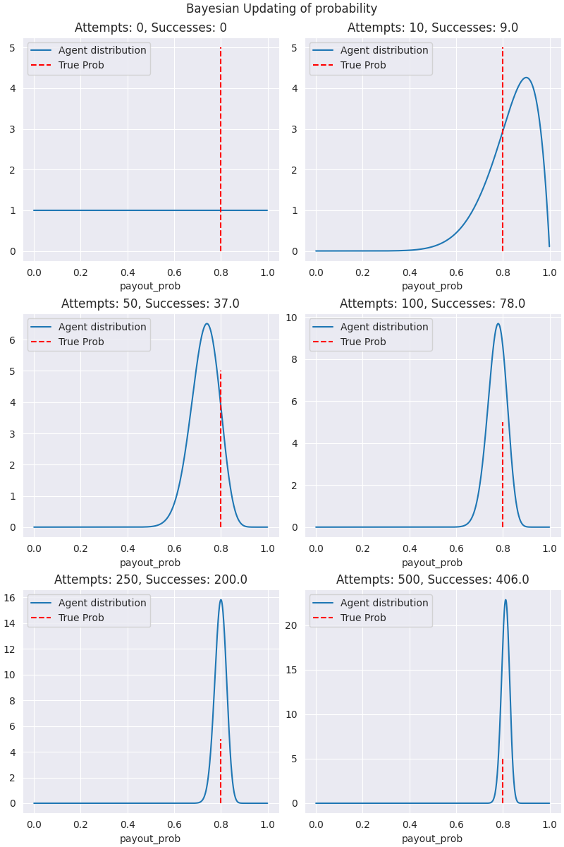 Here we can see that the agent has learned and honed in on the arm pretty effectively.
We can now develop a more sophisticated bandit and agent which will actually have to choose which arm to pull every run.
Setting up the bandit
Let us start with a 4 armed bandit where the probabilities are initialized randomly.
Import the required packages.
import tensorflow_probability as tfp
import tensorflow as tf
import pandas as pd
import numpy as np

tfd = tfp.distributions

print(tfp.__version__)
class BanditNoContext():
    """
    Non contextual Bernoulli bandit class which is instantiated with stationary
    probabiltities for each each arm

    Keyword Arguments:
        num_arms (int) - Number of arms the bandit has
        arm_probs (list) - List of true payout probabilities (0,1) that each arm
            has. Randomized if None.
    """
    def __init__(self, num_arms = 3, arm_probs = None):
        super(BanditNoContext, self).__init__()
        self.num_arms = num_arms
        self.arm_probs = arm_probs

        if not self.arm_probs:
            self.arm_probs = np.round_(
                [np.random.uniform(0, 1) for i in range(self.num_arms)],
                decimals=1
            )

    def action_arm(self, arm_id):
        """
        Pull an arm of the bandit and return the reward.

        Keyword Arguments:
            arm_id (int): Arm of bandit to pull.

        Returns
            reward: Binary value of the reward.
        """

        # Sample a Bernoulli distribution given the true probability of the
        # arm
        reward = tfd.Bernoulli(
                probs=self.arm_probs[arm_id],
                dtype=tf.float32,
                name='Bernoulli'
            ).sample().numpy()
        return reward

    def __repr__(self):
        return np.array_str(self.arm_probs)
This class instantiates a bandit with a set number of arms, each with a true probability of paying out. Let's start with a 4 armed bandit with probabilities [0.1, 0.3, 0.5, 0.8].
import BanditNoContext

probs = [0.1, 0.3, 0.5, 0.8]
bandit = BanditNoContext(num_arms=len(probs), arm_probs=probs)
We can try sampling each arm once to see what the rewards are.
for i, p in enumerate(probs):
    print(f"arm: i, prob: {p}, reward: {bandit.action_arm(arm_id=i)} \n")
arm: i, prob: 0.1, reward: 1.0

arm: i, prob: 0.3, reward: 0.0

arm: i, prob: 0.5, reward: 1.0

arm: i, prob: 0.8, reward: 0.0
Setting up the Agent
Like the bandit, we will set up and agent class. Rather than just keep track of the results, the agent will have to choose which arm to select. The agent class is given by
class AgentNoContext():
    """
    Agent which learns the probabilities and explores and exploits the arms of
    an associated bandit.

    Keyword Arguments:
        num_arms (int) - Number of arms to sample, explore and action. Should
            match the number of possibiliities of the bandit.
        hist_dict (dict) - Dictionary of agents history with the bandit. Tracks
            the total number of attempts and successes for each arm.
        total_reward (int) - Total number of successes across all arms.
        total_attempts (int) - Total number of attempts across all arms.
    """
    def __init__(self, num_arms):
        super(AgentNoContext, self).__init__()
        self.num_arms = num_arms
        self.hist_dict = {}
        for i in range(num_arms):
            self.hist_dict[i] = [0, 0]
        self.total_reward = 0
        self.total_attempts = 0


    def sample_arms(self):
        """
        Sample the each arm given the most recent prior distribution of the
        probabilities. This is modeled as a Beta function.

        Returns: The id of the arm with the highest sampled probability of
        payout.
        """

        samps = [] # Store samples in list
        for i in range(self.num_arms):
            # Define beta function based on historical successes.
            s = tfd.Beta(
                concentration1 = self.hist_dict[i][1] + 1, # a
                concentration0 = self.hist_dict[i][0] - self.hist_dict[i][1] + 1, # b
                force_probs_to_zero_outside_support=True,
                name = 'beta'
            ).sample().numpy()
            samps.append(s)

        return np.argmax(samps)

    def action_arm(self, arm_id, bandit):
        """
        Interact with the bandit. Select the arm to pull and recieve the
        associated reward.

        Keyword Arguments:
        arm_id (int) - arm of bandit to sample.
        bandit (Bandit class) - Instantiated bandit class to interact with.
        """
        return bandit.action_arm(arm_id)

    def action_agent(self, bandit):
        """
        Perform an action with the agent. This includes sampling, pulling the
        arm, and updating the statistics.

        Keyword Arguments:
        bandit (Bandit class) - Instantiated bandit class to interact with.
        """
        # print(self.hist_dict)
        arm_id = self.sample_arms()
        reward = self.action_arm(arm_id, bandit)
        self.total_reward += reward
        self.total_attempts += 1

        self.hist_dict[arm_id][1] += reward
        self.hist_dict[arm_id][0] += 1

    def __repr__(self):
        print(f"Total Reward: {self.total_reward}")
        print(f"Total Attempts: {self.total_attempts}")
        return repr(
            pd.DataFrame.from_dict(
                self.hist_dict,
                orient='index',
                columns=['attempts', 'successes']
            )
        )
This class instantiates an agent which will sample and learn the probability distribution of each of the arms using Thompson sampling.
Setting up an agent with the same number of arms as the bandit.
import AgentNoContext
agent = AgentNoContext(num_arms=bandit.num_arms)

print(agent)
   attempts  successes
0         0          0
1         0          0
2         0          0
3         0          0
Now, let's to a single run and see how the agent updates.
agent.action_agent(bandit)
agent
   attempts  successes
0         0          0
1         0          0
2         0          0
3         1          1
As you can see the last arm was sampled and there was a positive reward. This updated agent's statistics on final arm.
Thompson Sampling with a single parameter
To see how Thompson Sampling works, let's look closer at the sample_arms
method of the agent.
def sample_arms(self):
    """
    Sample the each arm given the most recent prior distribution of the
    probabilities. This is modeled as a Beta function.

    Returns: The id of the arm with the highest sampled probability of
    payout.
    """

    samps = [] # Store samples in list
    for i in range(self.num_arms):
        # Define beta function based on historical successes.
        s = tfd.Beta(
            concentration1 = self.hist_dict[i][1] + 1, # a
            concentration0 = self.hist_dict[i][0] - self.hist_dict[i][1] + 1, # b
            force_probs_to_zero_outside_support=True,
            name = 'beta'
        ).sample().numpy()
        samps.append(s)

    return np.argmax(samps)
This method is run at the start of every action and chooses which arm the agent will pull. In short it does the following: 1. Generate a Beta distribution for each arm using historical results. 2. Sample a value of the probability from each of the arms. 3. Select arm whose sample is the largest.
Initially, as all arms have uniform distribution, each arm has an equally likely chance of being selected. As the agent starts to update its probabilities, samples with higher mass for large probability values will be selected more than those with lower. We demonstrate this below.
Complete agent-bandit run
Using the same abndit and agent above (instantiated again), ee will do 1000 runs and plot the posterior distribution of the arm probability at each 100 iterations.
def plot_posterior(axs, bandit, agent, iteration):
    lin_x = np.arange(0, 1, 0.001)

    for arm_id in range(bandit.num_arms):
        a = agent.hist_dict[arm_id][1] + 1 # successes + 1
        b = agent.hist_dict[arm_id][0] - agent.hist_dict[arm_id][1] + 1 # failures + 1
        y = tfd.Beta(
            concentration1=a,
            concentration0=b,
        ).prob(lin_x)

        mean = np.round((a + b)/b, 1)
        successes = agent.hist_dict[arm_id][1]
        failures = agent.hist_dict[arm_id][0] - agent.hist_dict[arm_id][1]

        text = f"""
        mean_prob: {mean}
        s = {successes}
        f = {failures}
        """

        sns.lineplot(x=lin_x, y=y, ax=axs[arm_id])
        axs[arm_id].set_xlabel("payout_prob")
        axs[arm_id].set_title(f"Arm {arm_id} \n pulls: {agent.hist_dict[arm_id][0]}, successes: {agent.hist_dict[arm_id][1]}")
        axs[arm_id].vlines(x=bandit.arm_probs[arm_id], ymin=0, ymax=5, colors='r', linestyles='--')
import BanditNoContext, AgentNoContext

bandit = BanditNoContext(num_arms=4, arm_probs=[0.1, 0.3, 0.5, 0.8])
agent = AgentNoContext(num_arms=bandit.num_arms)

iterations=1001
nrows=math.floor(iterations/100) + 1
ncols=bandit.num_arms
print(nrows)

fig, axs = plt.subplots(nrows=nrows, ncols=1, constrained_layout=True, figsize=(ncols*4, nrows*6))
fig.suptitle('Bernoulli agent updating')

for ax in axs:
    ax.remove()

# add subfigure per subplot
gridspec = axs[0].get_subplotspec().get_gridspec()
subfigs = [fig.add_subfigure(gs) for gs in gridspec]

r=0
for i in range(iterations):
    if i%100 == 0:
        print(r)
        subfig = subfigs[r]
        subfig.suptitle(f'Iterations: {i}')
        axs = subfig.subplots(nrows=1, ncols=ncols)
        plot_posterior(axs, bandit, agent, iteration=i)
        r += 1
    agent.action_agent(bandit=bandit)
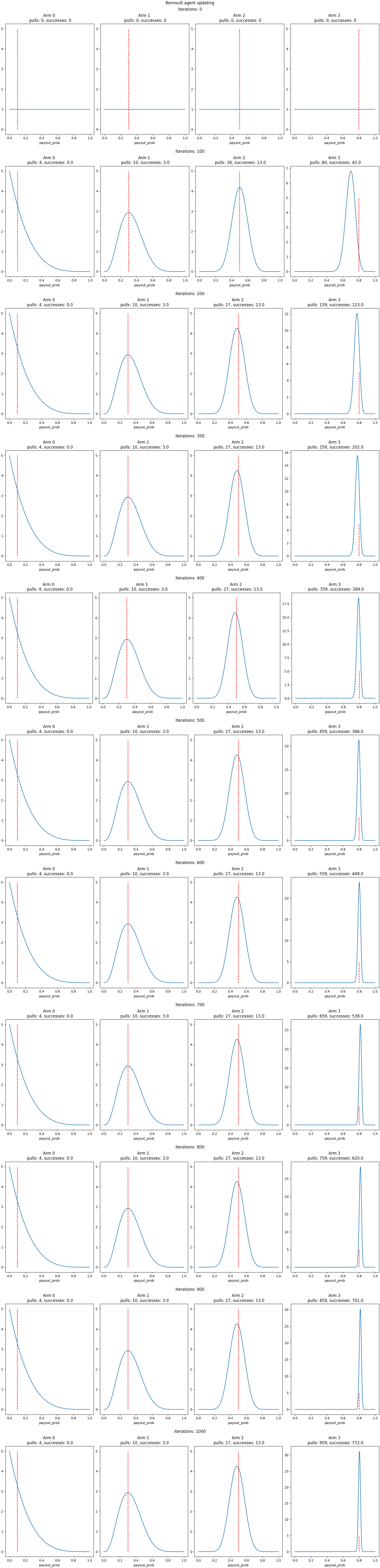
As you can see from the above plot, Thompson sampling does not aim to equally learn the probability distributions of each of the arms. In fact, it can seem to explore an insufficient amount as some arms only have few pulls and the upper probability has >95% of the pulls. This shows that the explore/exploit choice is built into Thompson sampling.
New we will use numerical approach to update the probability distribution of each arm.