Ames House Price Predictor

Kaggle Competition.

Models used to predict house prices based on a feature rich training set of Ames house sales. Based on the Kaggle competition "House Prices: Advanced Regression Techniques". This repo contains several models with differing levels of effectiveness.

Techniques

Feature Engineering
Forest Models
Regression Models
Boosting Models
Pipelines
Hyper-parameter Optimization
Model Interpretation

Exploration of the Data

To begin we do a preliminary assessment of the data. First we load the standard modules

import pandas as pd
import numpy as np

from matplotlib import pyplot as plt
import seaborn as sns

and load the data

## Load the training and testing data
    training_data = pd.read_csv(os.path.join(DATA_DIR, 'train.csv'), index_col = 'Id')
    test_data = pd.read_csv(os.path.join(DATA_DIR, 'test.csv'), index_col = 'Id')

As the data contains both numerical and categorical data it is important to get a count and list of these predictors,

## Count the number of numerical columns
numerics = ['int16', 'int32', 'int64', 'float16', 'float32', 'float64']
num_numeric = len(training_data.select_dtypes(include=numerics).columns)

## Count the number of object Columns
object_types = ['object']
num_objects = len(training_data.select_dtypes(include=object_types).columns)

## number of rows of the training set
num_rows = training_data.shape[0]

print("Total num of rows: ", str(num_rows))
print("Total num of columns: ", str(len(training_data.columns))
print("Num numerical of columns: ", str(num_numeric))
print("Num object of columns: ", str(num_objects))

Total num of rows: 1460
Total num of columns: 80
Num numerical of columns: 37
Num object of columns: 43

There is also some missing data in both the training and testing set and therefore we need to be careful with building our models as we may need to impute certain values.

To get an overview of the missing values and the number of unique values for each predictor (important for encoding decisions) we use the following,

## List of columns with nan values
na_col_list_train = [col for col in training_data.columns if training_data[col].isnull().any()]

na_col_dict_train = {}
for col in na_col_list_train:
    na_col_dict_train[col] = training_data[col].isna().sum()

## Catagorical Data
obj_col_dict_train = {}
for col in object_cols(training_data):
    obj_col_dict_train[col] = training_data[col].nunique()

print("### Catagorical Data \n")
print("Number of unique objects: " , str(obj_col_dict_train))

print("### Columns with nan values \n")
print("Columns with nan values: ", str(na_col_dict_train))

### Catagorical Data
Number of unique objects
{'MSZoning': 5, 'Street': 2, 'Alley': 2, 'LotShape': 4, 'LandContour': 4, 'Utilities': 2, 'LotConfig': 5, 'LandSlope': 3, 'Neighborhood': 25, 'Condition1': 9, 'Condition2': 8, 'BldgType': 5, 'HouseStyle': 8, 'RoofStyle': 6, 'RoofMatl': 8, 'Exterior1st': 15, 'Exterior2nd': 16, 'MasVnrType': 4, 'ExterQual': 4, 'ExterCond': 5, 'Foundation': 6, 'BsmtQual': 4, 'BsmtCond': 4, 'BsmtExposure': 4, 'BsmtFinType1': 6, 'BsmtFinType2': 6, 'Heating': 6, 'HeatingQC': 5, 'CentralAir': 2, 'Electrical': 5, 'KitchenQual': 4, 'Functional': 7, 'FireplaceQu': 5, 'GarageType': 6, 'GarageFinish': 3, 'GarageQual': 5, 'GarageCond': 5, 'PavedDrive': 3, 'PoolQC': 3, 'Fence': 4, 'MiscFeature': 4, 'SaleType': 9, 'SaleCondition': 6}

### Columns with nan values
{'LotFrontage': 259, 'Alley': 1369, 'MasVnrType': 8, 'MasVnrArea': 8, 'BsmtQual': 37, 'BsmtCond': 37, 'BsmtExposure': 38, 'BsmtFinType1': 37, 'BsmtFinType2': 38, 'Electrical': 1, 'FireplaceQu': 690, 'GarageType': 81, 'GarageYrBlt': 81, 'GarageFinish': 81, 'GarageQual': 81, 'GarageCond': 81, 'PoolQC': 1453, 'Fence': 1179, 'MiscFeature': 1406}

We also can use pandas describe and info methods to get statistical information on the numerical data. In the project folder, this information is populated into a file using exploration.py.

From this information we can conclude the following: * There are 1460 training observations.

From this we see that there are a total of 80 feature columns (and one predictor column in the training data). Of these, 37 are numerical and the remainder are categorical and therefore we will need to use an encoder to use them in our model.
Only the 'Neighbourhood' and 'Exterior*' features has a large number of unique categories which could prove difficult to encode if we choose to use them. The rest have roughly 4-5 categories.
'LotFrontage', 'Alley', 'PoolQC', 'Fence' and 'MiscFeature' all have a large number of nan values. For ambiguous features like 'LotFrontage' and 'MiscFeature' these amount of values are prohibitive and we will not use those features. Hoever for the other feauture we can infer meaning from the nan values. For instance a nan value in 'PoolQC' would probably mean there is no pool which we would expect to be a big factor in the price of the house. We will fix this feature later. We will also ignore the 'Fence feature'.

Plots and Feature Engineering

Correlation Matrix

Considering just the numerical columns it is informative to see which features are highly correlated with each other. We plot the correlation matrix,

columns = ['YearBuilt', 'OverallQual', 'OverallCond', 'LotArea',
'BedroomAbvGr', 'FullBath', 'HalfBath', 'GarageCars', 'PoolArea', 'Fireplaces',
'YearRemodAdd', 'GrLivArea', 'TotRmsAbvGrd', 'TotalBsmtSF', 'SalePrice']

correl = data[columns].corr()

fig, ax = plt.subplots(nrows=1, ncols=1, figsize=(12,12))
ax.set_title("Correlation matrix of numerical predictors")
sns.heatmap(data=correl, annot=True, cmap="YlGnBu", square=True, ax=ax)

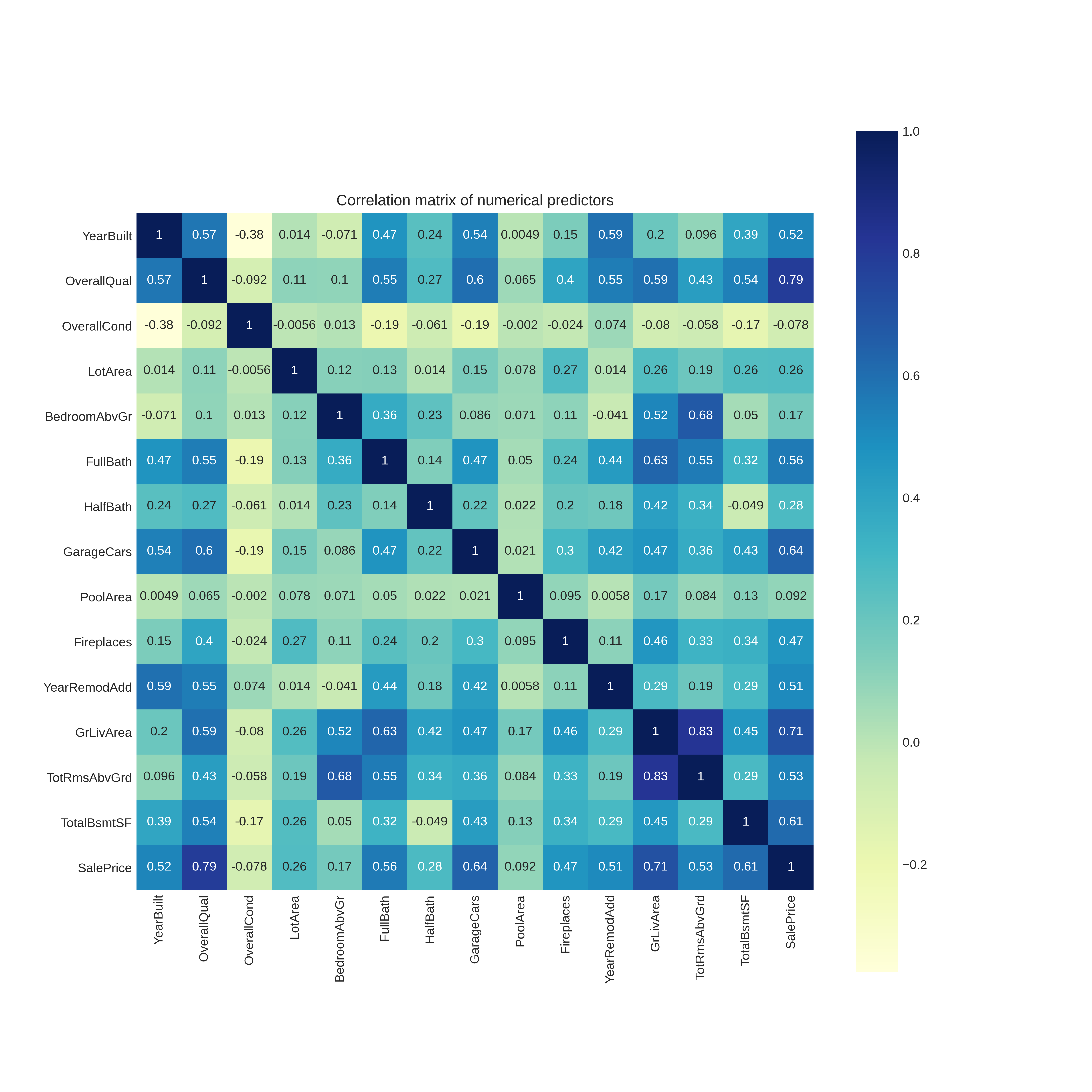
Looking at the bottom row of this matrix we can determine which numerical predictors are most correlated with SalePrice. As expected, the most correlated are,

Overall Quality
Ground Living Area
Garage Cars
Total Basement Area (Square feet)
Year Built

Surprisingly however it seems the overall condition and pool area does not correlate with the house sales price.

Distribution plots

It is important to see the distributions of the target (SalePrice) and predictors to see if there are any data irregularities.

columns = ['YearBuilt', 'OverallQual', 'OverallCond', 'LotArea',
    'BedroomAbvGr', 'FullBath', 'HalfBath', 'GarageCars', 'Fireplaces',
    'YearRemodAdd', 'GrLivArea', 'TotRmsAbvGrd', 'TotalBsmtSF', 'SalePrice']

    fig, ax = plt.subplots(nrows=5, ncols=3)
    for idx, col in enumerate(columns):
        sns.distplot(data[col], ax=ax[int(idx/3),idx % 3], rug=True)

From these distribution plots we can see there are some anamalous datapoints which may negatively affect the performance of our model.

There are sparse data points with LotArea > 100000 square feet. These may be rural properties.
There are sparse datapoints with GrLivArea > 5000.
There is an anomalous point with TotalBsmtSF > 6000.
Some SalePrice datapoints above $700000.

We will identify and remove these data points (They can be added in later to see if they have any impact on the model),

print("Lot Area anomalous points")
print(data[data['LotArea'] > 100000]['Id'].to_string(index=False))
print("Ground Area anomalous points")
print(data[data['GrLivArea'] > 5000]['Id'].to_string(index=False))
print("Basement Area anomalous points")
print(data[data['TotalBsmtSF'] > 6000]['Id'].to_string(index=False))
print("Saleprice anomalous points")
print(data[data['SalePrice'] > 700000]['Id'].to_string(index=False))

Lot Area anomalous points
 250
 314
 336
 707
Ground Area anomalous points
1299
Basement Area anomalous points
1299
Saleprice anomalous points
692

Therefore we drop these from the training data and reindex the dataframe

training_data = training_data.drop(training_data[training_data['Id'] == 1299].index)
training_data = training_data.drop(training_data[training_data['Id'] == 250].index)
training_data = training_data.drop(training_data[training_data['Id'] == 314].index)
training_data = training_data.drop(training_data[training_data['Id'] == 336].index)
training_data = training_data.drop(training_data[training_data['Id'] == 707].index)
training_data = training_data.drop(training_data[training_data['Id'] == 629].index)

training_data.set_index('Id')

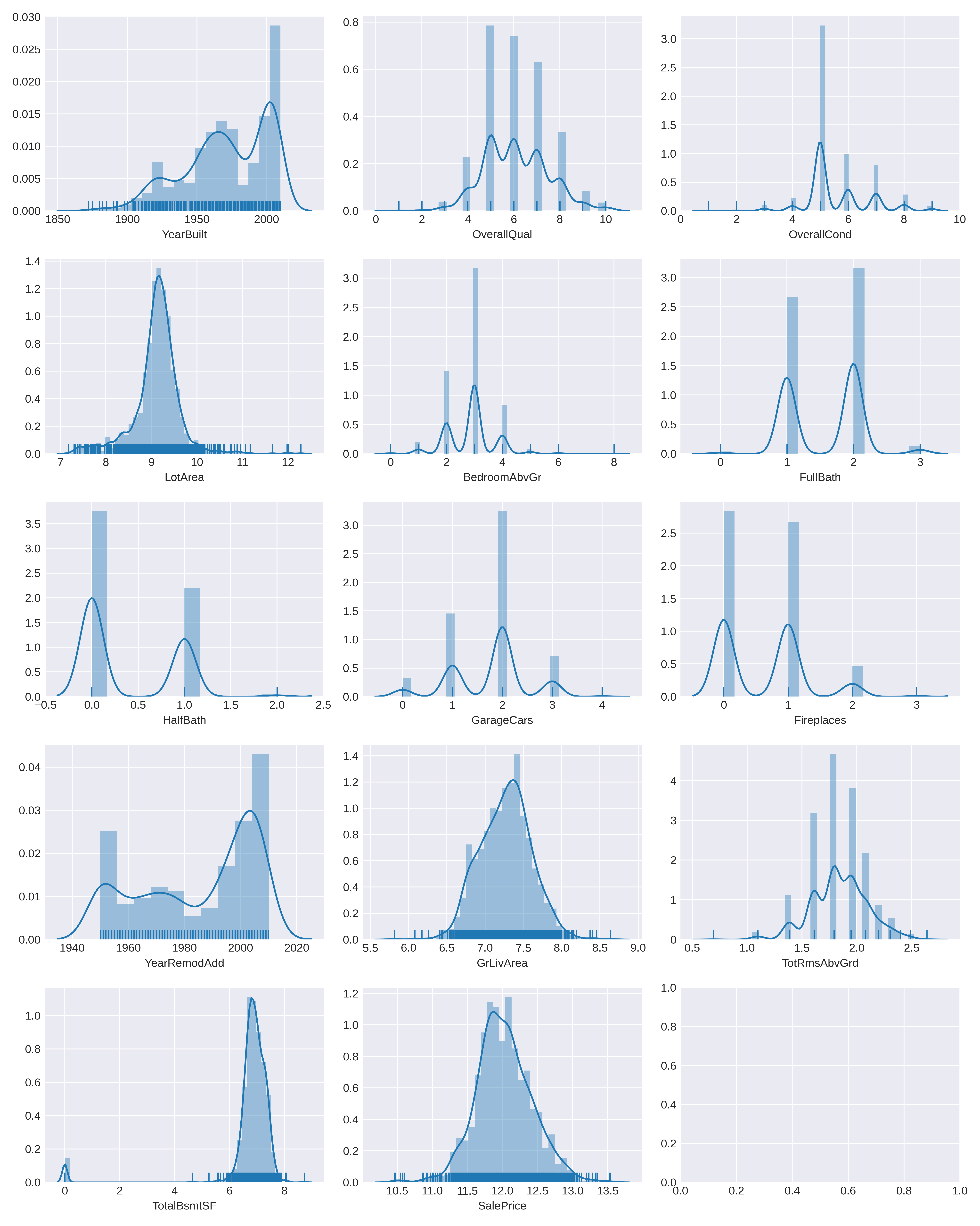
Another thing to note from the distribution plots is the clear skew in several of the predictors and the target. Specifically in LotArea, GrLivArea, SalePrice and TotalBsmtSF.

These look like lognormal distributions so we will log transform them. However, for TotalBsmtSF there are values of zero and therefore can't just log the raw values. We will create a new predictor HasBsmt to indictor whether there is a basement $1$ or no basement "0".

training_data['HasBsmt'] = pd.Series(len(training_data['TotalBsmtSF']), index=training_data.index)
training_data['HasBsmt'] = 0
training_data.loc[training_data['TotalBsmtSF']>0,'HasBsmt'] = 1

Now for all properties with basement we will log transform the data,

training_data.loc[training_data['HasBsmt']==1,'TotalBsmtSF'] = np.log(training_data['TotalBsmtSF'])

and simply log transform the other variables,

training_data['SalePrice'] = np.log(training_data['SalePrice'])
training_data['GrLivArea'] = np.log(training_data['GrLivArea'])
training_data['LotArea'] = np.log(training_data['LotArea'])
training_data['TotRmsAbvGrd'] = np.log(training_data['TotRmsAbvGrd'])

This produces the new plots,

Lastly, we will create a new feature HasPool to indicate whether the house has a pool or not,

training_data['has_pool'] = training_data.apply(lambda x: 0 if x['PoolArea'] == 0 else 1, axis = 1)

This is all for the numerical data. To see that there is no missing values left we will do a recheck of the dataframe,

nan_numeric = training_data[['YearBuilt', 'OverallQual', 'OverallCond', 'LotArea',
    'BedroomAbvGr', 'FullBath', 'HalfBath', 'GarageCars', 'Fireplaces',
    'YearRemodAdd', 'GrLivArea', 'TotRmsAbvGrd', 'TotalBsmtSF', 'SalePrice']].isna().sum()
print(nan_numeric)

YearBuilt       0
OverallQual     0
OverallCond     0
LotArea         0
BedroomAbvGr    0
FullBath        0
HalfBath        0
GarageCars      0
Fireplaces      0
YearRemodAdd    0
GrLivArea       0
TotRmsAbvGrd    0
TotalBsmtSF     0
SalePrice       0

We will deal with the categorical nan values with the onehot encoder in the pipeline.

Model Approach

The repository of this project has several approaches to this regression problem, using decision trees and random forests. These approaches are good for learning and reference. Here we will only present the pipeline approach which will demonstrate the simplicity and versitility of pipeline.

Scoring

We will set a scoring function for our pipeline as the square root of the mean squared error (RMSE) between the preditions and true values. As we have log transformed out prices this represent the RMSE of the log prices.

from sklearn.metrics import mean_squared_error, make_scorer

log_score = np.abs(np.sqrt(mean_squared_error(y_valid, predictions)))
custom_score = make_scorer(log_score, greater_is_better=False)

Set up data for modeling

Using the training dataframe processed above, split into predictors (X) and target (y)

numeric_features = ['YearBuilt', 'OverallQual', 'OverallCond', 'LotArea',
'BedroomAbvGr', 'FullBath', 'HalfBath', 'GarageCars', 'Fireplaces',
'YearRemodAdd', 'GrLivArea', 'TotRmsAbvGrd', 'TotalBsmtSF', 'HasBsmt', 'HasPool']
object_features = ['CentralAir', 'LandContour', 'BldgType',
'HouseStyle', 'ExterCond', 'Neighborhood']
scale_features = ['YearBuilt', 'GrLivArea', 'TotRmsAbvGrd', 'LotArea', 'BedroomAbvGr']
features = numeric_features + object_features

X = training_data[features]
y = training_data['SalePrice']

The pipeline

The pipeline will have the following steps,

One-hot encode the categorical variable and scale the features with standard scaler
Reduce the dimensions of the feature space with Principle Component Analysis (PCA)
Fit an XGBoost model

Another benefit of the pipeline is it will allow us to optimize the hyper-parameters in both the model and the preprocessing. We can easily implement a cross-validated random grid search.

Define the transformer

We define a ColumnTransformer which selectively transforms the categorical features and numerical features to be scaled,

from sklearn.compose import ColumnTransformer
from sklearn.preprocessing import StandardScaler, OneHotEncoder

transformer = ColumnTransformer(transformers=[
                                   ('scaler', StandardScaler(), scale_features),
                                   ('oh_encode', OneHotEncoder(handle_unknown='ignore'), object_features),
                                   ], remainder='passthrough')

Define the hyperparameter space to test

import scipy.stats as stats

one_to_left = stats.beta(10, 1)
from_zero_positive = stats.expon(0, 50)

params_list = []

## reduce_dim parameters (PCA)
PCA_parameters = {'reduce_dim': [PCA()],
                'reduce_dim__n_components': n_features_to_test,
                }

## XGBoost parameters
XGB_params = {"XGboost__n_estimators": stats.randint(3, 40),
            "XGboost__max_depth": stats.randint(3, 40),
            "XGboost__learning_rate": stats.uniform(0.05, 0.4),
            "XGboost__colsample_bytree": one_to_left,
            "XGboost__subsample": one_to_left,
            "XGboost__gamma": stats.uniform(0, 10),
            'XGboost__reg_alpha': from_zero_positive,
            "XGboost__min_child_weight": from_zero_positive,
            }

params_list.append(dict(**PCA_parameters, **XGB_params))

Instantiate the Pipeline

from sklearn.pipeline import Pipeline
import xgboost as xgb
from sklearn.decomposition import PCA

pipe = Pipeline([
        ('transform', transformer),
        ('reduce_dim', PCA()),
        ('XGboost', xgb.XGBRegressor(objective='reg:squarederror'))
        ])

The pipeline can be run with default hyperparameters though we will use cross-validation

Instantiate and fit Random Grid Search with the estimator as the pipeline

Perform the cross validated random search to identify the best hyperparameters to use. n_iter denotes the number of searches to run

randsearch = RandomizedSearchCV(estimator=pipe, param_distributions=params_list, verbose=1, scoring=custom_score, n_iter=10000, n_jobs=-1).fit(training_data[features], training_data[target])

Print the best cv score for the training set and the best hyperparameter:

## Print the best score from the search
    cv_score = randsearch.best_score_
    print('cv-score: ' + str(round(cv_score, 4)))

An example output of this is,

[Parallel(n_jobs=-1)]: Done 50000 out of 50000 | elapsed:  5.7min finished
cv-score: 0.157
Score on validation set: 0.1017
Best Parameters for XGBoost:
{'XGboost__colsample_bytree': 0.9650585840453798, 'XGboost__gamma': 0.09349135571176559, 'XGboost__learning_rate': 0.39802053325159514, 'XGboost__max_depth': 10, 'XGboost__min_child_weight': 20.489255763052462, 'XGboost__n_estimators': 23, 'XGboost__reg_alpha': 0.22614299594203852, 'XGboost__subsample': 0.9957300822116487, 'reduce_dim': PCA(copy=True, iterated_power='auto', n_components=19, random_state=None,
    svd_solver='auto', tol=0.0, whiten=False), 'reduce_dim__n_components': 19}

Saving and loading the model

To save from performing the cross-validated search again or saving the parameters for future fitting it is convenient to save the model as a pickle and load the pickle when you need to use it again,

def save_model(model, model_name, cv_score, model_params):
    """
    Saves model to the model directory (creates one if it does not already exist).
    """
    ## Create model directory with title case if one does not exist.
    if not os.path.exists(os.path.join(MODEL_DIR, model_name.title())):
        os.makedirs(os.path.join(MODEL_DIR, model_name.title()))

    ## Save the model the in this directory with filename model_name.sav.
    model_file = open(os.path.join(os.path.join(MODEL_DIR, model_name.title()), model_name + '.sav'), 'wb')
    pickle.dump(model,  model_file)
    model_info = open(os.path.join(os.path.join(MODEL_DIR, model_name.title()), 'model_info.txt'), 'w')
    model_info.write('cv-score :' + cv_score + '\n\n')
    model_info.write('best parameters :' + model_params + '\n\n')
    model_info.write(str(model) + '\n\n')
    model_info.close()
    model_file.close()
    print("Model successfully saved.")

def load_model(model_name):
    """
    Loads the specified model.
    """
    model_location = os.path.join(os.path.join(MODEL_DIR, model_name.title()), model_name + '.sav')
    print(model_location)
    model_file= open(model_location, 'rb')
    model = pickle.load(model_file)
    model_file.close()
    print("Model successfully loaded.")

    return model

Model Evaluation

An important part of machine learning is model explanability. Therefore this repo includes codes to evaluate which features of the model have the largest affect. These are included in 'model_evaluation.py'. In terms of a single summary statistic, the best score these models produced on the Kaggle leaderboard is: 0.14175 from the Root-Mean-Squared-Error of the logarthims.

Future development

I have seen interesting work on using only feature engineering and regularized linear regression to model this data extremely well. The next step in this project will be to build a streamlined pipeline using only linear models to see if a model with a large bias and low variance could model this data well.