Disaster tweets

The impetus and data used for this project was from this Kaggle Competition

About

This objective of this competition is to use NLP methods to determine if a tweet is about a natural disaster or not (a two class classification problem). A large training data set of ~ 7000 tweets is supplied and a testing set for submission.

Data Exploration

As this is a classification problem the ratio of the target variables is important. If there is a large class imbalance, then when we split the data for training and validating we need to ensure we have a representative amount of each target.

This is not a problem with our dataset as there are roughly the same number of 'Disaster' tweets (target = 1) and 'No Disaster' (target = 0).

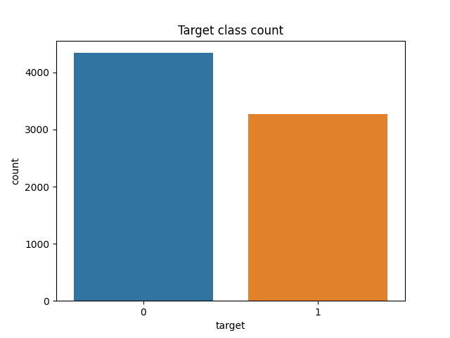
Figure 1: Count plot of the target varaibles. '1' corresponds to a disaster related tweet and '0' otherwise.

We also look at the word count distribution of the tweets to see if there are any outliers or abnormalities. As a defining characteristic of tweets is their limits length, there should not be any large outliers. Below are the total length (character count) and word count distributions of the training and test sets

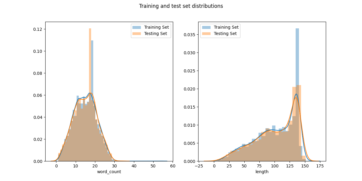
From these distributions we see that the the training and test sets have near identical distributions of length. This is excellent as it makes it more likely the training set is a good representation of the test set.

Now we will see if there is a difference in distributions between the target classes. This is shown in the following plot:

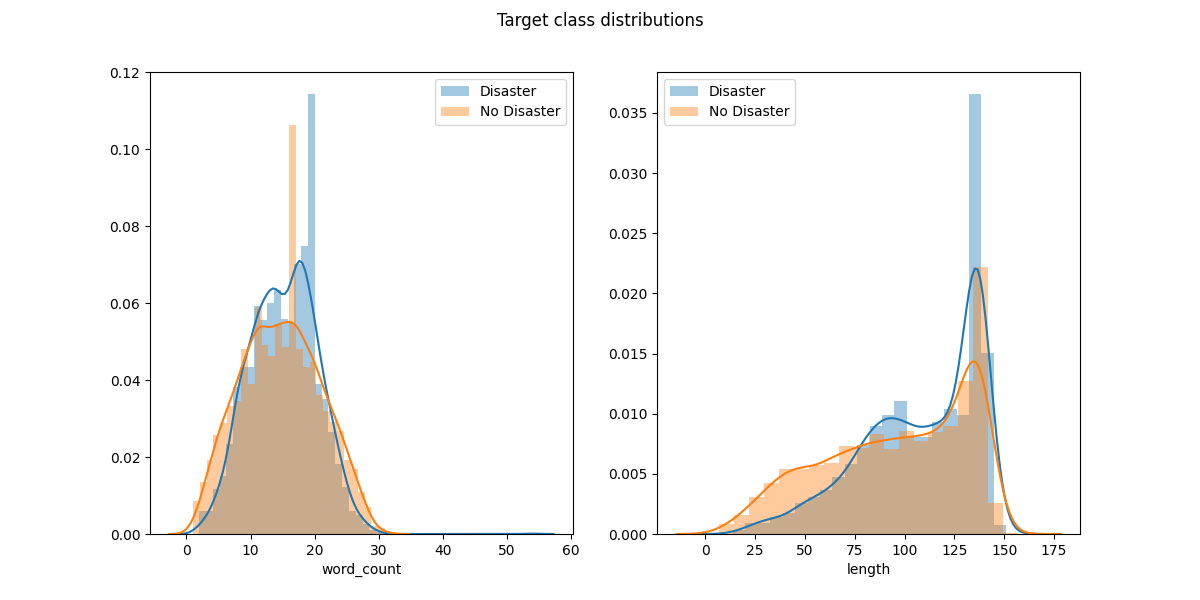
We can see that, surprisingly, the distribution of word counts and total lengths are similar for each class. Therefore a crude classification scheme based on length and word count will be ineffective.

Models

As this project is primarily for learning I will present several different approaches to traning and predicting the nature of tweets with different techniques. The first approach is the 'bag of words' approach.

For each model we load the data into pandas dataframes with

train_df = pd.read_csv(os.path.join(DATA_DIR, "train.csv"), index_col="id")
test_df = pd.read_csv(os.path.join(DATA_DIR, "test.csv"), index_col = 'id')

Bag of Words

NLP frequency based approach where each sentence is broken down into an unordered vector depending on how many times a specific word appears. This method does not preserve the order of the sentence or consider the semantic structure of the sentence.

In bag of words each separate 'document' (in this case tweet) is tokenized by seperating the sentence into individual components such as words and punctuation. These tokenized documents can then be normalized by removing stopwords, stemming etc.

After normalizing the data a count matrix is generated for each document. Each row of this matrix corresponds to each document in the corpus and the number of columns corresponds to the number of unique words in the entire corpus (order of tens of thousands). In the basic bag of words model the matrix is populated with integers based on how many times each word occurs in each document. This results in an incredibly sparse matrix in our case with tweets.

Below I use two separate BoW approaches. The scripts can be found in 'bow.py'

Sklearn approach

First we present the most simplistic count vectorizer model with a naive Bayes classifier.

We need to load the following modules

import pandas as pd
import numpy as np

from sklearn.metrics import f1_score, classification_report
from sklearn.model_selection import train_test_split, cross_val_score
from sklearn.feature_extraction.text import CountVectorizer, TfidfTransformer
from sklearn.naive_bayes import MultinomialNB
from sklearn.pipeline import Pipeline

import string
import nltk
from nltk.corpus import stopwords

First we need to process the text for learning, as seen above there is no need to remove any outliers or anomalous tweets for training though we will need to clean up the tweets themselves. While sklearn's CountVectorizer has inbuilt text preprocessing we will define our own processing function here for demonstration. We will remove the punctuation from the text and remove the stopwords from each tweet. We have a function which will clean up each tweet and return a list of the cleaned text.

def text_process(mess):
    """
    Takes in a string of text, then performs the following:
    1. Remove all punctuation
    2. Remove all stopwords
    3. Returns a list of the cleaned text
    """
    # Check characters to see if they are in punctuation
    nopunc = [char for char in mess if char not in string.punctuation]

    # Join the characters again to form the string.
    nopunc = ''.join(nopunc)

    # Now just remove any stopwords
    return [word for word in nopunc.split() if word.lower() not in stopwords.words('english')]

Here we use the nltk package to identify and remove the stopwords. For example, this function will clean tweet 19,

tweet_19 = train_df.loc[19]['text']
print('Original Tweet: ', tweet_19)
tweet_19_cleaned = text_process(tweet_19)
print('Processed Tweet: ', tweet_19_cleaned)

Original Tweet:  #Flood in Bago Myanmar #We arrived Bago
Processed Tweet:  ['Flood', 'Bago', 'Myanmar', 'arrived', 'Bago']

We can see that it removed the hashtags and stopwords such as 'We'. Now as we are considering tweet removing the hashtags may not be the wisest approach as it normally identifies the keywords of the tweet. We will consider keeping them later on.

Using just this we can build a simple BoW pipeline with Naive Bayes classification.

pipeline = Pipeline(steps = [('bow_transformer', CountVectorizer(analyzer=text_process)),
                            ('mnb', MultinomialNB())
                            ])

To evaluate this model we can run a 5-fold cross validation with F1 scoring.

## Set the features and predictors
X = train_df['text']
y = train_df['target']

## Define scoring parameters for cross vaidation
scoring = {'f1': 'f1_macro', 'Accuracy': make_scorer(accuracy_score)}
CV = cross_validate(pipeline, X, y, cv=5, scoring=scoring, verbose=1, n_jobs=1)

## Print the scores
print("Cross-Validation Accuracy: {0:.3} \n \
Cross-Validation F1 Score: {1:.3}".format(CV['test_Accuracy'].mean(), CV['test_f1'].mean()))

Cross-Validation Accuracy: 0.707
Cross-Validation F1 Score: 0.697

This simple model will classify approximately 70% of tweets correctly. While this is better than random chance, it is still quite a low score and more sophisticated text processing and training needs to be considered. To determine whether another classification scheme may given better results without more normalization we can run our pipeline with a variety of different models.

## Define a dictionary all the desired classifiers.
classifier_dict = {'MNB':MultinomialNB(),
                   'LSVC':LinearSVC(dual=False),
                   'poly_SVM':SVC(kernel='poly', C=100),
                   'sig_SVM':SVC(kernel='sigmoid', C=1.00),
                   "RBF_SVM":SVC(gamma=0.0001, C=1000000.0)}

## Run a loop over each classifier which outputs the cv scores
for key, value in classifier_dict.items():
    print("Classifier " + key)
    pipeline = Pipeline(steps = [('bow_transformer', CountVectorizer(analyzer=text_process)),
                                (key, value)
                                ])
    CV = cross_validate(pipeline, X, y, cv=5, scoring=scoring, verbose=0, n_jobs=1)
    # print(CV)
    print("Cross-Validation Accuracy: {0:.3} \n \
    Cross-Validation F1 Score: {1:.3}".format(CV['test_Accuracy'].mean(), CV['test_f1'].mean()))

Classifier MNB
Cross-Validation Accuracy: 0.707
Cross-Validation F1 Score: 0.697

Classifier LSVC
Cross-Validation Accuracy: 0.665
Cross-Validation F1 Score: 0.641

Classifier poly_SVM
Cross-Validation Accuracy: 0.586
Cross-Validation F1 Score: 0.412

Classifier sig_SVM
Cross-Validation Accuracy: 0.691
Cross-Validation F1 Score: 0.653

Classifier RBF_SVM
Cross-Validation Accuracy: 0.655
Cross-Validation F1 Score: 0.63

The SVM hyperparameters might increase the scores but not by a significant amount. After further preprocessing we will optimize these hyperparameters with a randomized search.

Normalize all tokens to a similar case

A small improvement may be to normalize the document so all tokens are lower case. The text_process function will be:

def text_process(mess):
    """
    Takes in a string of text, then performs the following:
    1. Remove all punctuation
    2. Remove all stopwords
    3. Returns a list of the cleaned text
    """
    # Check characters to see if they are in punctuation
    nopunc = [char for char in mess if char not in string.punctuation]

    # Join the characters again to form the string.
    nopunc = ''.join(nopunc)

    # Now just remove any stopwords
    return [word.lower() for word in nopunc.split() if word.lower() not in stopwords.words('english')]

We will only test the MultinomialNB classifier. We have a new cross-validation score of:

Cross-Validation Accuracy: 0.722
Cross-Validation F1 Score: 0.704

and we already have an increase of 1%. This is not significant though further processing can be made.

Stemming words

'Stemming' refers to the reduction of words into a base form. This can significantly reduce the size of the vocabulary as many like words will be reduced into a single lemma.

To stem our tweets we include another step in our text_process function.

def text_process(mess):
    """
    Takes in a string of text, then performs the following:
    1. Remove all punctuation
    2. Remove all stopwords
    3. Stem words.
    4. Returns a list of the cleaned text in lowercase
    """
    # Check characters to see if they are in punctuation
    nopunc = [char for char in mess if char not in string.punctuation]

    # Join the characters again to form the string.
    nopunc = ''.join(nopunc)

    # Now just remove any stopwords
    word_list = [word for word in nopunc.split() if word.lower() not in stopwords.words('english')]

    # Lowercase all the words
    word_list = [word.lower() for word in word_list]

    # Stem words
    porter = PorterStemmer()
    stemmed = [porter.stem(word) for word in word_list]

    return stemmed

To see how this affects the text ttake the same tweet as above for example:

Original Tweet:  #Flood in Bago Myanmar #We arrived Bago
Processed Tweet:  ['flood', 'bago', 'myanmar', 'arriv', 'bago']

Interestingly, this had no large affect on the CV Accuracy using MNB classifier

Most common words for each classification

As we have built the BoW model it is interesting to look at the most common words for each classificiation. This will also help us in identifying and removing any anomalous words. To generate the word count for the entire set of tweets

bow = CountVectorizer(analyzer=text_process)
bow.fit(X)
X_bow = bow.transform(X)
word_count = pd.Series(data=X_bow.toarray().sum(axis=0), index=bow.get_feature_names()).sort_values(ascending=False)
print("Words which appear most: \n", word_count.head(50))
print("Words which appear least: \n", word_count.tail(50))

There seems to be no anomalous words which appear frequently. On the other hand, there are a large number of anomalous 'words' which only appear once. For example words starting with 'http' are common. Let's remove those by adding the following to the text_process function.

# Remove pattern matched words
pattern = '^http\w*'
pat = re.compile(pattern)
word_list = [word for word in word_list if not pat.match(word)]

This will remove any words beginning with 'http'. Running the lowest frequency words counts will show you that these have been removed. Now it is interesting to see which words appear most for each of the classifications.

bow = CountVectorizer(analyzer=text_process)
bow.fit(X)

total_wc = pd.Series(data=X_bow.toarray().sum(axis=0), index=bow.get_feature_names()).sort_values(ascending=False)
disaster_wc = pd.Series(data=disaster_bow.toarray().sum(axis=0), index=bow.get_feature_names()).sort_values(ascending=False)
no_disaster_wc = pd.Series(data=no_disaster_bow.toarray().sum(axis=0), index=bow.get_feature_names()).sort_values(ascending=False)

fig, ((ax1), (ax2), (ax3)) = plt.subplots(nrows=3, ncols=1, figsize=(12,18))

plt.suptitle("Most Frequent Words")

sns.barplot(x=total_wc[0:30].values, y=total_wc[0:30].index, ax=ax1)
ax1.set_title("Complete Training Set")

sns.barplot(x=disaster_wc[0:30].values, y=disaster_wc[0:30].index, ax=ax2)
ax2.set_title("Disaster Tweets")

sns.barplot(x=no_disaster_wc[0:30].values, y=no_disaster_wc[0:30].index, ax=ax3)
ax3.set_title("Non Disaster Tweets")

plt.show()

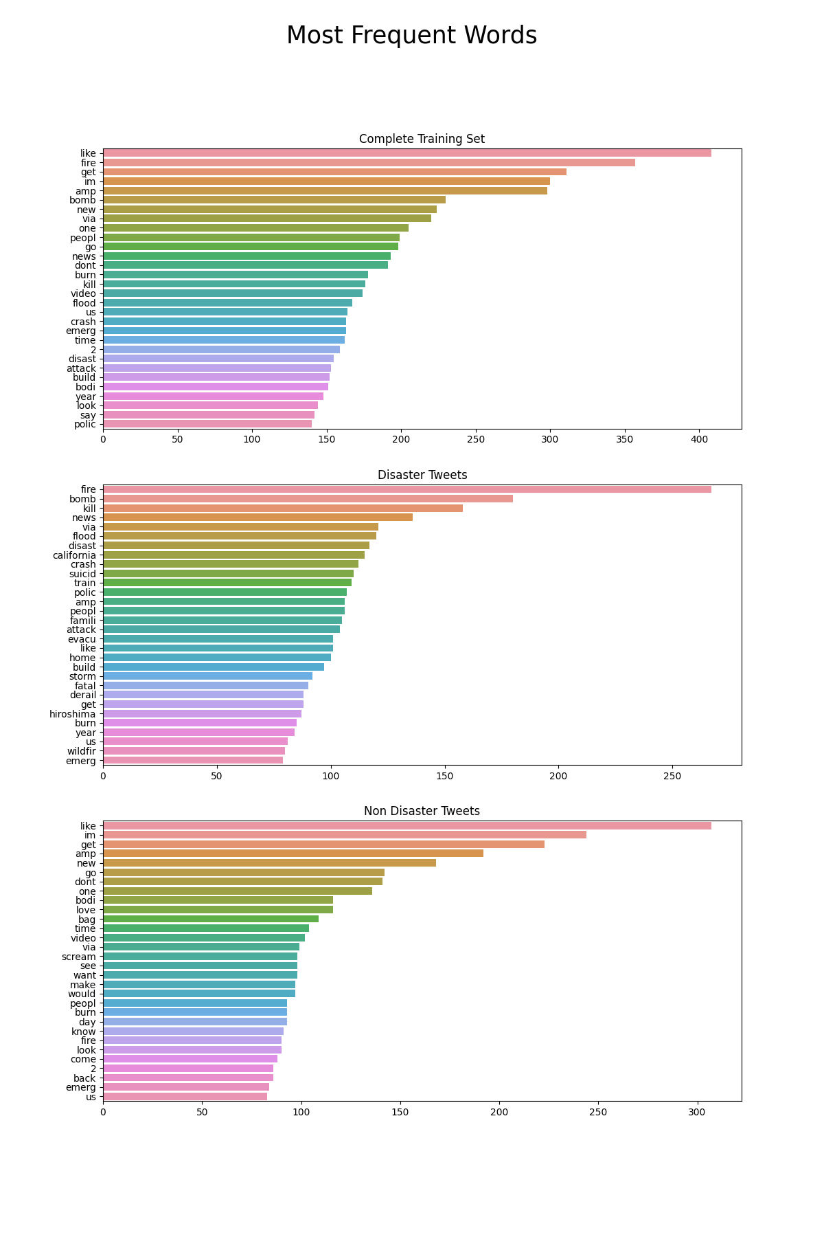
In general no words in particular stick out as anomalous. Lastly, we will see which of the most common words are common between the two sets. We find the list of words in the top 100 most frequent for disaster and non disaster.

disaster = set(disaster_wc.index[0:100])
common = [word for word in no_disaster_wc.index[0:100] if word in disaster]
print(len(common))

There are 36 common words in the top 100 from each list.

Hyper-parameter Optimization

After preprocessing it is important to optimize the hyperparameters of the pipeline.

spaCy text categorizer

SpaCy is a powerful nlp module which takes into account the semantic content of texts not just the frequency of words. This is quite powerful as it can differentiate between meanings of words from their context in the sentence and building a model can therefore perform much better.

The spaCy module performs a lot of the same steps in tokenizing the text. After the text has been tokenized, it is parsed through a pipe and compared to a vocabulary to further categorize each of the tokens. Below we will present a simple text categorization model using spacy.